Temporal predictive regression models
for linguistic style analysis
Carmen Klaussner and Carl Vogel School of Computer Science and Statistics,
Trinity College Dublin
abstract
Keywords: language change, style analysis, regression
This study focuses on modelling general and individual language change over several decades. A timeline prediction task was used to identify interesting temporal features. Our previous work achieved high accuracy in predicting publication year, using lexical features marked for syntactic context. In this study, we use four feature types (character, word stem, part-of-speech, and word n-grams) to predict publication year, and then use associated models to determine con-stant and changing features in individual and general language use. We do this for two corpora, one containing texts by two different authors, published over a fifty-year period, and a reference corpus containing a variety of text types, representing general language style over time, for the same temporal span as the two authors. Our linear regression models achieve good accuracy with the two-author data set, and very good results with the reference corpus, bringing to light interesting features of language change.
1
introduction
analy-sis is known as synchronic analyanaly-sis, as it disregards composition or publication dates.
However, this is a simplification, since most writers compose over time spans of 20–40 years, where they not only undergo individual stylistic development, but also bear witness to general contempora-neous language change. These two types of temporal influences can cause synchronic analyses to be misinterpreted. Thus, as already dis-cussed by Daelemans (2013), unless style is found to be invariant for an author and does not change with age and experience, temporality can be a confounding factor in stylometry and authorship attribution. For this reason, diachrony presents an important aspect of style anal-ysis, not only to disambiguate synchronic analyses of style, but also in its own right by modelling language change over time.
In this work, we examine language change in two literary authors, as well as the corresponding background language change during the same time period. Specifically, we are interested in features that are attested in each time slice of the diachronic corpus studied. We refer to this subset of features that appear in all samples as ‘constant’ features. This classification captures occurrence patterns rather than variation in terms of relative frequencies, which may or may not change over the time intervals examined. In order to identify salient constant features that exhibit change over time, we refer to a temporal prediction task based on the features’ relative frequencies.
This extends our previous work on predicting the publication year of a text using syntactic word features (Klaussner and Vogel 2015).1 That study considered a data set comprising works by two authors from the 19thto the 20thcentury, as well as a data set based on a ref-erence corpus, and sampled features that appeared in many, but not necessarily all, time slices. For the two-author data set, a root-mean-square error (RMSE) of 7.2 years2on unseen data (baseline: 13.2) was
1These are lexical features that have been marked for syntactic function to differentiate between lexical representations that can appear in different syntac-tic contexts (see Section 4.2).
obtained, whereas the model built on the larger reference data set ob-tained an RMSE of 4 on unseen data (baseline: 17). While the current work is similar in that it uses the same data sets and the same gen-eral prediction task, it is different in that achieving ‘high accuracy’ of prediction is not the main objective here. Although we report our results and compare them to those from the earlier study, the pre-diction task is primarily used as a means to determine what is stable and what changes in individual and general language use over time.3 Hence, the purpose is not the pursuit of a perfect temporal classifier, but rather to understand ‘typical’ distributions of linguistic feature cat-egories during an author’s lifetime. This change must also be under-stood in relation to the effects of ageing on language production, as explored for instance by Pennebaker and Stone (2003). Features that are not constant in the sense analysed here are also important. We focus on constant features, because if they are used in each time slice throughout an author’s career, then they are probably integral to that author’s style, making the relative frequencies of such features across time slices interesting to explore.
The contribution of this new study is the analysis of language change using an extended feature set, adding character,4word stem, and syntactic (part-of-speech tag) features to the previous set, which consisted only of syntactic word features. In addition, rather than con-sidering only unigram size, this study analyses all n-gram sizes up to length four. Therefore, one of the questions investigated as part of this work is whether (and to what extent) the more linguistically informa-tive features, such as syntactic word n-grams, exhibit more dramatic change than lexicographic and part-of-speech features. We present our own method for reasoning about temporal change in constant linguis-tic features, using standard techniques from regression analysis, par-ticularly parameter shrinkage.5We find that the best predictive values common to the works by the two authors and the reference corpus are word stem, and POS bigrams and trigrams, which also account for
most shared model predictors. In terms of language change, with the help of our regression models, we identified several differences be-tween the reference corpus and the works by the two authors.
The remainder of this article is structured as follows: Section 2 outlines previous work in the area; Section 3 discusses methods; Sec-tion 4 presents the data sets, preprocessing steps, and feature types; Section 5 discusses the general experimental setup and the experi-ments themselves. Section 6 reports and analyses the salient features of the models. Section 7 discusses the results, and Section 8 concludes this work.
2
related work
the closed-candidate setting, reducing the number of candidates im-proves accuracy (e.g. 1,000 candidates yields 93.2% precision with 39.3% recall), whereas in the open-class setting, having fewer candi-dates actually introduces problems, in that an author might end up being chosen erroneously, because there is less competition. Overall, Koppel et al.(2011) find that their methods achieve passable results even for snippets as short as 100 words, but note that there is still no satisfactory solution for the case of a small open-candidate set and limited anonymous text.
Another general variant of the attribution problem is commonly referred to as ‘Authorship verification’, which requires determining whether a piece of text has been written by a specific author. This has been considered by Koppel et al.(2007), for instance, who show that the task of deciding whether an author has written a particular text can be accurately determined by iteratively removing the set of best features from the learning process: the differences between two texts by the same author are usually only reflected in a relatively small number of features, causing accuracy to drop much faster and more dramatically than when the texts were not written by the same per-son. In contrast, ‘Author profiling’, which involves predicting an au-thor’s characteristics, such as gender, age or personality traits, based on a particular text, has been studied extensively as part of the PAN competitions (e.g. see Rossoet al.2016). While the predicted variable varies by task, what is common to the studies above as well as to our own is the use of relative frequencies of some feature to predict the variable of interest, using similarity-based or statistical methods.
pro-portion of hapax legomena, and repetition of frequently appearing vocabulary. In addition to testing the constancy of these properties over time, weighted linear regression is used to test associations be-tween these measures and the time of a play’s first performance. For this, the property’s value in a particular text block is used as re-sponse, and time of performance is used as predictor.6Results show that Aristophanes’ use of hapax legomena appears to have decreased over time. Interestingly, one of his earlier works, Clouds, which was subjected to redrafting after the first staging, but for which the fin-ishing date is unknown, is predicted to originate towards the end of the playwright’s life, indicating that revisions might have been made at a much later stage. Our work here also uses linear regres-sion, but rather than using time as predictor, we investigate to what extent pooled information from several features can accurately pre-dict a text’s publication year. The study presented by Hoover (2007) considers language change in Henry James’ style with respect to the 100–4,000 most frequent word unigrams, using methods such as ‘Cluster Analysis’, ‘Burrows’ Delta’, ‘Principal Component Analy-sis’, and ‘Distinctiveness Ratio’.7 Three different divisions, into early (1877–1881), intermediate (1886–1890), and late style (1897–1917), emerge from the analysis.8 However, rather than being strict divi-sions, there seem to be gradual transitions, with the first novels of the late period being somewhat different from the others, suggest-ing that it might be interestsuggest-ing to conduct a continuous analysis of style in James’ works. Thus, in contrast to the previous study, the work we present here focuses on a more graduated interpretation of style over time, with yearly intervals rather than classification into
6In order to perform inverse prediction, i.e. predicting the date of an un-known work by the measure, the authors draw a horizontal line at y, withy
corresponding to the measure’s average in the text and look at the intersection with the estimated regression line.
7Distinctiveness Ratio: Measure of variability defined by the rate of occur-rence of a word in a text divided by its rate of occuroccur-rence in another. Principal Component Analysis (PCA) is an unsupervised statistical technique to convert a set of possibly related variables to a new uncorrelated representation, i.e., prin-cipal components.
different periods along the timeline of the author’s works. Our work on temporal prediction (Klaussner and Vogel 2015) considered the task of accurately predicting the publication year of a text through the relative frequencies of syntactic word features.9 We used multi-ple linear regression models to predict the year when a text was pub-lished, for three data sets, the first containing texts by Mark Twain and Henry James, the second a mid 19th to early 20th century ref-erence corpus, and a third one combining all data from the previ-ous two sets. Although the data for the two authors had been kept separate to allow for potentially different levels between them, the models disregarding authorial source tended to be more accurate (RMSE of 7.2 vs. 8.0). While the reference corpus model performed well on its own test set (RMSE of 4), using it to predict publica-tion year for the two authors was rather inaccurate (RMSE: 15.4 for Twain, and 20.3 for James). This suggests that the style of the two authors was rather different from general language, Twain’s being somewhat more similar to it than James’. Combining all data leads to more accurate results (RMSE: 1.8), and model features and esti-mates suggest a marked influence of Twain and James on the model, in spite of their smaller data sets (for more detailed, quantitative re-sults, see Section 5.3).
On the topic of suitable stylistic feature types in this context, Sta-matatos (2012) compares the performances of the most frequent func-tion words and character trigrams for the authorship attribufunc-tion task. It is shown that character trigrams outperform word features, espe-cially when training and test corpus differ in genre – they are also found to be more robust and effective when considering different fea-ture input sizes. For this reason, we include character n-grams as a feature type here as well. In contrast to part-of-speech tags or word stems, character n-grams present a less linguistically motivated fea-ture type, as writers would not be able to control the number of times a particular character is used to the same extent as they would be able to control their choice of particular syntactic constructions. Yet this feature type becomes more likely to bear meaning, as character n-gram size increases, approaching average word length.
3
methods
This section discusses the methods used in this work, beginning with temporal regression models (Section 3.1), and continuing with evalu-ation techniques for these predictive models (Section 3.2).
3.1 Temporal regression models
The analysis of data over time probably has its most prominent usage in quantitative forecasting analysis, which involves the (quantitative) analysis of how a particular variable (or variables) may change over time and how that information can be used to predict its (or their) fu-ture behaviour, thus inherently assuming that some aspects of the past continue in the future, known as the ‘continuity assumption’ (Makri-dakis et al.2008). Thus, a future value of a variable y is predicted
using a function over some other variable values. These other variable values could be composed in two different ways, pertaining either to the use of a ‘time-series’ model or an ‘explanatory’ model. When con-sidering a time-series model, the assumption is that one can predict the future value of the variable y by looking at the values it took at
previous points in time and the possible patterns this would show over time. In contrast, for prediction, explanatory models focus less on in-terpreting previous values of the same variable, and more on the rela-tionship with other variables at the same point in time. Consequently, the prediction of a variable y, using explanatory models, is based on
a function over a set of distinct variables:x1,x2, . . . ,xp−1,xp=X, with
y ∈/ X, at the same time point t:{t∈1, . . . ,n}, and some error term: yt=f(x1t, . . . ,x2t, . . . ,xp−1t, . . . ,xpt,error).
The general model for this is shown in Equation (1), predicting variable y, where ˆyt refers to the estimate of that variable at a
partic-ular time instance t:{t∈1, . . . ,n}, β0refers to the intercept, and βp
to the pth coefficient of thepth predictor xpt.
(1) ˆyt=β0+β1x1t+β2x2t+· · ·+βpxpt
In the present case, the year of publication is always set as the re-sponse variable, so that a model based on syntactic unigrams (relative frequencies) for the year 1880 could be defined in the following way:
ˆ
y1880=β0+β1(N N1880) +β2(N P1880) +β3(I N1880).
model and observed values yi, the RSS measures the difference
be-tween them. The smaller the RSS, the greater the amount of variation of y values around their mean that is explained by the model. This
is known as the ‘ordinary least squares’ (OLS) fit, a model selection criterion that also forms the basis of evaluation measures, such as the root-mean-square error (RMSE) (see Section 3.2).
In this work, rather than applying models based only on least squares regression, we employ so-called ‘shrinkage’ models that offer an extension to regular OLS models by additionally penalizing coeffi-cient magnitudes, thus aiming to keep the model from overfitting the data. Specifically, we use the ‘elastic net’, which is a combination of the two most common types of shrinkage, ‘lasso’ and ‘ridge’ regres-sion (Zou and Hastie 2005). The elastic net penalizes both the L1and L2norms,10 causing some coefficients to be shrunk (ridge) and some
to be set to zero (lasso), with the exact weighting between the two also being subject to tuning. In addition, the elastic net tends to select groups of correlated predictors rather than discarding all but one from a group of related predictors, as is common when using only the lasso technique. The entire cost function is shown in Equation (2). As with the lasso and ridge regression, λ≥0 controls finding a compromise between fitting the data and keeping coefficient values as small as possible, while the elastic net parameterαdetermines the mix of the two penalties, i.e. how many features are merely shrunk as opposed to being completely removed.
(2) max
{β0,k,βk∈R p}K
1
∑N
i=1
log Pr(gi|xi)−λ K ∑
k=1
p ∑
j=1
(α|βk j|+ (1−α)βk j2)
There are numerous advantages to using shrinkage models, and the elastic net estimation in particular, such as built-in feature selec-tion and more robust and reliable coefficient estimaselec-tion. This is dis-cussed in more detail for instance by Jameset al.(2013, pp. 203–204) and Friedmanet al.(2001, pp. 662–663).
3.2 Evaluation
The ‘root-mean-square error’ (RMSE) is one of the measures that can be used for the purpose of evaluating linear regression models: it is
10∥β∥ 1:
∑
i|βi|and∥β∥22:
∑ iβ
2
defined as the square root of the variance of the residuals between outcome and predicted value and thus provides the standard deviation around the predicted value, as shown in Equation 3.
(3) RMSE=
v u
t∑n
t=1(ˆyt−yt)2
n
The advantage over the more general ‘mean-square error’ (MSE) is that RMSE computes deviations in predictions on the same scale as the data. However, due to the squaring, assigning more weight to larger errors, the RMSE is more sensitive to outliers.
4
data
The following section presents the data sets (Section 4.1), followed by feature types (Section 4.2), and finally, data preparation (Section 4.3).
4.1 Data sets
The data for this study originates from three separate sources: works by two American authors, Mark Twain and Henry James, and a refer-ence corpus for American English, from 1860 to 1919.
both individual and general language change are of interest in their own right, they also provide comparative information about the rela-tive importance of the features observed, indicating whether particu-lar events are likely to be unusual.
For each of the two authors, we compiled a separate data set of their main works.11 Table 1 shows the data for Henry James, and Table 2 that for Mark Twain. The texts were collected from theProject Gutenberg12 and the Internet Archive13 selecting the earliest editions available. The reference corpus was assembled by taking an extract fromThe Corpus of Historical American English(COHA; Davies 2012).14 The COHA is a 400-million-word corpus, containing samples of Ameri-can English from 1810–2009, balanced in size, genre and sub-genre in each decade (1,000–2,500 files each). It contains balanced language samples from fiction, popular magazines, newspapers and non-fiction books, which are again balanced across sub-genres, such as drama and poetry.15The COHA data were compiled from different sources, some of which were already available as part of existing text archives (e.g.,
Project Gutenberg andMaking of America), whereas others were con-verted from PDF images, or scanned from printed sources. The corpus allows analysis of linguistic change at different levels, i.e. lexical, mor-phological, syntactic, and semantic.
4.2 Feature types
For the experiments described in Section 5, we consider four dif-ferent types of features, as well as various sequence sizes of these. Table 3 lists all feature types, ordered by increasing degree of speci-ficity, with an example for unigrams, and one for trigrams.
The most general type is character n-grams, including punctu-ation and single spaces.16 While the character n-grams reduce words
11In this case, ‘main’ is with reference to the size of the work in kilobytes, rather than in terms of literary importance. We use kilobytes instead of word count, as this gives a more precise indication of file size.
12http://www.gutenberg.org/– last verified March 2018. 13https://archive.org/– last verified March 2018.
14Free version available from:http://corpus.byu.edu/coha/– last veri-fied March 2018.
15An Excel file with a detailed list of sources is available from: http:// corpus.byu.edu/coha/– last verified March 2018.
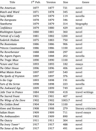
Table 1: Collected works for Henry James. Showing ‘Title’, the original publica-tion date (‘1stPub.’), version collected (‘Version’), ‘Size’ in kilobytes and ‘Genre’ type. The dashed lines indicate the boundaries for compression, i.e. which of the works are combined into one temporal interval (see Section 4.3 for discussion of the compression technique used)
Title 1stPub. Version Size Genre
The American 1877 1877 721 novel
Watch and Ward 1871 1878 345 novel
Daisy Miller 1879 1879 119 novella
The Europeans 1878 1879 346 novel
Hawthorne 1879 1879 314 biography
Confidence 1879 1880 429 novel
Washington Square 1880 1881 360 novel
Portrait of a Lady 1881 1882 1200 novel
Roderick Hudson 1875 1883 750 novel
The Bostonians 1886 1886 906 novel
Princess Casamassima 1886 1886 1100 novel
The Reverberator 1888 1888 297 novel
The Aspern Papers 1888 1888 202 novella
The Tragic Muse 1890 1890 1100 novel
Picture and Text 1893 1893 182 essays
The Other House 1896 1896 406 novel
What Maisie Knew 1897 1897 540 novel
The Spoils of Poynton 1897 1897 376 novel
In the Cage 1893 1898 191 novella
Turn of the Screw 1898 1898 223 novella
The Awkward Age 1899 1899 749 novel
Little Tour in France 1884 1900 418 travel writings
The Sacred Fount 1901 1901 407 novel
The Wings of the Dove 1902 1902 1003.7 novel
The Golden Bowl 1904 1904 1100 novel
Views and Reviews 1908 1908 279 literary criticism
Italian Hours 1909 1909 711 travel essays
The Ambassadors 1903 1909 890 novel
The Outcry 1911 1911 304 novel
The Ivory Tower* 1917 1917 488 novel
The Sense of the Past* 1917 1917 491 novel
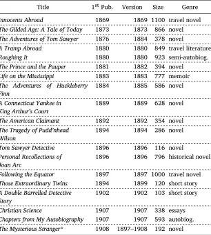
Table 2: Collected works for Mark Twain. Showing ‘Title’, the original publication date (‘1stPub.’), version collected (‘Version’), ‘Size’ in kilobytes and ‘Genre’ type. The dashed lines indicate the boundaries for compression, i.e. which of the works are combined into one temporal interval (see Section 4.3 for discussion of the compression technique used)
Title 1stPub. Version Size Genre
Innocents Abroad 1869 1869 1100 travel novel
The Gilded Age: A Tale of Today 1873 1873 866 novel
The Adventures of Tom Sawyer 1876 1884 378 novel
A Tramp Abroad 1880 1880 849 travel literature
Roughing It 1880 1880 923 semi-autobiog.
The Prince and the Pauper 1881 1882 394 novel
Life on the Mississippi 1883 1883 777 memoir
The Adventures of Huckleberry Finn
1884 1885 586 novel
A Connecticut Yankee in King Arthur’s Court
1889 1889 628 novel
The American Claimant 1892 1892 354 novel
The Tragedy of Pudd’nhead Wilson
1894 1894 286 novel
Tom Sawyer Detective 1896 1896 116 novel
Personal Recollections of Joan Arc
1896 1896 796 historical novel
Following the Equator 1897 1897 1000 travel novel
Those Extraordinary Twins 1894 1899 120 short story
A Double Barrelled Detective Story
1902 1902 103 short story
Christian Science 1907 1907 338 essays
Chapters from My Autobiography 1907 1907 593 autobiog.
The Mysterious Stranger* 1908 1897–1908 192 novel
‘*’ indicates unfinished works.
Table 3:
Feature types n-gram type Example
unigram trigram
character 〈c〉 〈ca,〉
part-of-speech (POS) 〈NP〉 〈IN DET NP〉
word stem 〈allud〉 〈to allud to〉
syntactic word (lexical) 〈like.IN〉 〈like.VB the.DET others.NNS〉
to’ or ‘alludes to’.17 The most specific is termed ‘syntactic word’ se-quences, meaning words that have been marked for syntactic class, as in the case of ‘like’, which may be used as a preposition or a verb, depending on context. CompareI’m like my father.andI like my father.: in the first instance ‘like’ is used as a preposition, in the second it is used as a verb. Hence, for this feature type, each word is given the cor-rect part-of-speech tag, thus allowing distinct features to be identified for words with more than one syntactic context, such as〈like.VB〉for verbal usage and〈like.IN〉 for prepositional usage.
4.3 Data preparation
Before features could be extracted from the two authors’ texts, each file had to be checked manually, to remove parts that were written at a different time from the main work, or introductions or comments not by the author, such as notes or introductions by editors. Follow-ing this, all source files were then searched (both automatically and manually) to remove unwanted formatting sequences and to normal-ize spacing.18
To extract both POS and syntactic word features, we used the TreeTagger POS tagger (Michalke 2014; Schmid 1994). The original word plus its tag is retained for syntactic word features, while for POS features, the original word is replaced by the POS tag.19After
ex-17The feature remains orthographic inasmuch as the stem differs from the lemma.
18The packagestylo(Ederet al.2013) was used to convert words into character sequences, while theRTextToolspackage (Jurkaet al.2012) was used to extract word stems.
traction, all feature types were then transformed to lowercase, as for this work we do not analyse features with respect to sentence bound-aries. Finally, document-feature matrices were constructed for each type and n-gram size and relativized in the following way: for all of the analyses reported here, we compute relative frequencies to take into account any differences in the amount of text available for each year.20If more than one work was available for a particular year and authorial source, they were joined together and relativized as one text. For both the reference set and the two-author set, an ordinal variable ‘year’ was added for each experiment to mark the publication year of a text. The data sets for the two authors were joined into one set after relativization, with an additional categorical variable ‘author’ to mark which author composed the text. In some instances, both authors pub-lished work during the same year; the ‘author’ variable served to keep such cases separate. Thus, detecting differences in levels of relative frequency by author remains possible within the joint data set. Com-bined relativization might distort individual interpretation or create a shift towards the author with more data in a given year. The model is trained on ‘combined’ data, in the sense that there may be two relative frequencies contributing observations to one predictor variable. The categorical author variable may be added to the model, if the level for that predictor differs between James and Twain.
5
experiments
Section 5.1 addresses general experimental design, and model and pa-rameter selection. The four feature types described in Table 3 are con-sidered separately for the two data sets hereafter, with Section 5.2 presenting the results, and Section 5.3 comparing them with the pre-vious study.
5.1 Model computations
Before the experiments, the same procedure was performed for all of the previously constructed document-feature matrices, to construct
the input for each of the 32 models shown in Table 5. The data were first divided into training and test data using a 75/25 stratified split on the ordinal variable ‘year’ that we added at the previous step.21 Af-ter that step, we extracted all constant features from the training set, i.e. the features appearing in all training set instances, which were then passed to the elastic net models.22
The final model was then computed by performing 10-fold cross-validation on the training data to find the ‘best’αandλparameters, deciding to what extent features were either shrunk or removed from the model as part of the elastic net configuration.23 We defined the ‘best’ α and λ parameter estimates for a model as their combined global optimum. This optimum was then defined as the most parsi-monious model within 1 standard error (SE) of the model with the lowest error, as defined by the MSE. By not choosing the best per-forming model, we could circumvent models that might be needlessly complex and thus somewhat balance prediction accuracy and model complexity. The evaluation parameter, RMSE, for the training and in-ternal test set was computed by taking the model MSE and computing its square root. For evaluation on external data, we had to rebuild the training model manually from the model’s coefficients.24 Occa-sionally, the sets of constant features differed across training and (ex-ternal) test sets, requiring us to add empty columns modelling ‘zero occurrence’ in the test data.
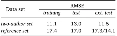
Table 4 shows the baseline results for both data sets. These re-sults are computed by using the mean of the data for prediction of every instance. The columns ‘training’ and ‘test’ refer to the 75/25 split of the data set. For the last column (‘ext. test’), the two previous
21This was done using thecaretpackage in R (Kuhn 2014).
22All regression models were computed using theglmnetpackage in R (Fried-manet al.2010), which in our opinion currently offers the most transparent and flexible implementation.
23The procedure followed was that outlined by Nick Sabbe: http://stats.stackexchange.com/questions/17609/
cross-validation-with-two-parameters-elastic-net-case – last verified: March 2018
Data set RMSE
training test ext. test
two-author set 11.1 13.0 11.5
[image:17.482.59.254.68.129.2]reference set 17.4 17.0 17.3/14.1
Table 4:
Baseline for both data sets
columns are added together to be used as an external validation set: i.e. the two-author model is validated on the reference data set and vice versa. There are two baselines for the reference set: the first one was calculated over the entire set, whereas the second one was based only on those items within the same time span as the two authors. Testing the two-author model on the smaller reference sample avoids extrapolation beyond the authors’ time span.
5.2 Model results
Based on the four feature types and four n-gram lengths, sixteen dif-ferent models were computed for each data set. Table 5 shows the model results for both the reference corpus (columns 2–7) and the two-author data set (columns 8–13). The first two columns for each set show the number of constant features compared to the total num-ber of features present for each feature type and n-gram length, giv-ing the raw counts as well as the correspondgiv-ing proportions.25 Con-sidering these proportions with respect to feature type and sequence length (i.e. unigram, bigram, trigram, or tetragram), one can observe several patterns with respect to the number of features extracted. For both data sets, the number of all features extracted increases with n-gram size for all four feature types. However, when considering only constant features, there is a difference for the more general character and POS types as opposed to the more specific stem and lexical types. While the general types always increase in cardinality but not in pro-portion in the next higher sequence, e.g. unigram to bigram, across all levels, the specific types only increase up to bigram/trigram size and then decrease again. In addition, the increase in total types is consid-erably higher and causes the proportion of constant types of all types to be much smaller than for the first group. This is undoubtedly due to the large number of extremely rare features, adding to the count of
total but not constant features. These patterns are primarily observ-able in the two-author data set, and are a little less pronounced for the reference data set. The remaining four columns for each set show training, test, and external test set RMSE, and the complexity of the model measured by the count ofβ coefficients.26
5.2.1 Reference corpus
We first consider models specific to the reference corpus, noting base-line results of 17.4 (training), 17.0 (test) and 11.5 (external test), as shown in Table 4. From the results in Table 5, one can observe that for character n-grams, model accuracy ranges from 2.9 to 4.5 years for the training set and from 2.8 to 5.2 years for the test set. Models ‘Char-2’ and ‘Char-3’ are best at balancing accuracy of pre-diction and model parsimony. With an RMSE of 20.9, ‘Char-1’ per-forms best on the two-author data, although this is still far from the baseline of 11.5, with the other three models being even less accurate (RMSE: 35–80). This suggests that there is little similar-ity between the data sets with regard to character n-grams. The re-sults for the syntactic sequences (POS-n) are very regular over all four n-gram sizes, varying between an RMSE of 3.3–4.3 years for the training set and 3.5–4.4 years for the test set. External valida-tion error on the two-author data set is lower than for the charac-ter n-grams but still not comparable with the baseline (18.5–21.4). Model complexity increases noticeably with n-gram size: our ‘POS-1’ model achieves an accuracy of 4.3 on the training set and 4.4 on the test set. While the bigram model ‘POS-2’ decreases this to 3.5 for both sets, it also adds 73 more predictors. Similarly, ‘POS-3’ and ‘POS-4’ both obtain an RMSE of 3.3 on the training set, but use 297 and 207 predictors, respectively. The word stem unigram and bigram models perform slightly better than their POS counter-parts, with model accuracy slightly deteriorating after that, despite using more predictors. ‘Stem-1’ and ‘Stem-2’ achieve 3.9 and 3.5 on the training set, with 3.2 for both on the test set. This deteriorates to 4.5 and 3.9 for ‘Stem-3’ and then to 5.1 and 5.6 for ‘Stem-4’. Exter-nal validation is better than for the two previous types (12.8–21.7), but still cannot quite compete with the baseline. Overall, syntactic
word features (Lex-n) and ‘Lex-1’, and ‘Lex-2’ in particular, yield the most accurate models. The unigram and bigram models obtain an er-ror of 2.8–2.9 on the training set and 2.2–3.0 on the test set. ‘Lex-1’ might be considered the best model overall, as it has 53 fewer pre-dictors than ‘Lex-2’, yet performs only slightly less well on the train-ing and test sets (0.1 and 0.8 years, respectively). The external val-idation error (17–20.6) is higher than for stem n-grams, indicating that the two data sets might be ‘closest’ for that type. As previously noted, some of the above models seem rather complex and, given the tendency of elastic nets to select correlated predictors, poses the question of whether so much complexity is needed to achieve model accuracy.
In order to see which models have a large number of correlated predictors, we consider the corresponding uncorrelated models by rerunning the same experiments, but using only the lasso method, i.e. setting α to 1. This highlights several aspects of the regression models computed earlier: a simple model of ∼10–30 predictors can still be improved by adding features, in the sense that these con-tribute enough new information to improve prediction accuracy. In most cases, however, adding more features to a model of 80 pre-dictors rarely improves prediction accuracy. Compare adding 7 fea-tures to achieve a −0.3/−0.5 error decrease (‘Lex-4’) to adding 151 features for a −0.5/−0.5 RMSE decrease (‘Lex-3’) for training set and test set respectively. What is also notable is that most lower n-gram models do not have any correlated predictors, seeing that elas-tic net and lasso methods yield the same models, whereas the num-ber of correlated predictors rises with n-gram size up to trigram size, whereafter model size suddenly decreases more or less dramatically.27 This strongly suggests that there is most overlap for trigram models on the most changing features used in each time slice. Thus, while there is likely to be most background language change in syntac-tic word features, all types produce accurate enough models to sug-gest that reasonably interesting temporal change must have taken place. The language change aspect is examined in more detail in Section 6.
5.2.2 Two-author data set
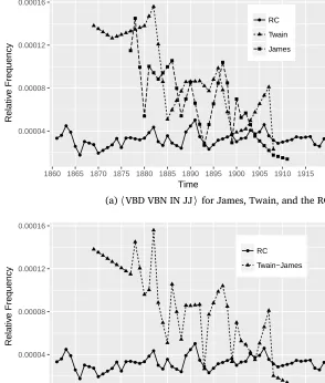
We now turn to the models intended to capture individual change, specifically in James’ or Twain’s language. The baseline results for the two authors yielded 11.1 (training), 13.0 (test) and 17.3/14.1 (exter-nal test). Beginning with the character n-gram models, Table 5 shows that ‘Char-1’ and ‘Char-2’ are very close to the baseline, containing very few predictors, indicating that these two types carried little dis-criminatory power. The trigram model ‘Char-3’ is the best character model, with 10/10.7 RMSE for training and test set, where the error is much lower than the baseline of 13, especially for the test set. The ‘Char-4’ model does not quite reach the same accuracy, although it is an improvement on the first two models. The results on the exter-nal test data are consistently congruent with the baseline for that set. Moving on to syntactic sequences, the unigram model ‘POS-1’ is actu-ally the null model, as it is the most parsimonious model within one standard error of the best model with 38 features, suggesting that this type is not discriminatory enough in relation to publication year. The best POS model is ‘POS-2’ with 10.2/8.3 on training and test set re-spectively, but it increases complexity by adding 69 predictors. ‘POS-3’ adds even more complexity (94 predictors), but performs worse than ‘POS-2’. Interestingly, the 94 predictors in ‘POS-3’ have the same predictive power on the training set as ‘POS-4’s one and only predic-tor〈VBD VBN IN JJ〉.28
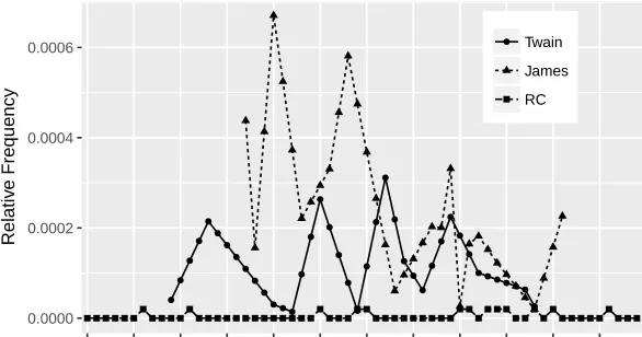
Figure 1 depicts the tetragram〈VBD VBN IN JJ〉 for Twain and James individually (Figure 1a) and combined together (Figure 1b). Even though relative frequency values vary over only a small range (0.00004–0.00016) for both James and Twain (Figure 1a), there is a discernible downward trend over time, offering a fair indication of temporal origin. The combined plot, though a generalization, still presents a fair approximation of each individual plot. In comparison, the same feature exhibits less of a trend over time for the reference corpus. The prediction accuracy of stem models is comparable to that of character and POS n-grams, while models tend to be more parsi-monious. Results range from 9.9–10.4 on the training set and 8.8–
Figure 1: The development over time of the tetragram〈VBD VBN IN JJ〉, showing relative frequency in relation to all tokens for the reference corpus (RC) and for the two authors. Figure (a) shows the feature for Twain and James separately. Figure (b) shows the combined two-author frequency, averaged for years when both published work ●● ● ● ● ● ● ●● ●● ●● ● ● ● ● ● ● ● ● ● ● ● ● ● ●● ● ● ● ● ● ●● ● ●● ●●● ● ● ● ● ● ● ● ● ●● ● ● ● ● ● ● ● ● 0.00004 0.00008 0.00012 0.00016
1860 1865 1870 1875 1880 1885 1890 1895 1900 1905 1910 1915 Time Relativ e Frequency ● RC Twain James
(a)〈VBD VBN IN JJ〉 for James, Twain, and the RC
●● ● ● ● ● ● ●● ●● ●● ● ● ● ● ● ● ● ● ● ● ● ● ● ●● ● ● ● ● ● ●● ● ●● ●●● ● ● ● ● ● ● ● ● ●● ● ● ● ● ● ● ● ● 0.00004 0.00008 0.00012 0.00016
1860 1865 1870 1875 1880 1885 1890 1895 1900 1905 1910 1915 Time
Relativ
e Frequency
● RC
Twain−James
(b)〈VBD VBN IN JJ〉for James + Twain, and the RC
10.2 on the test set for ‘Stem-1’, ‘Stem-2’ and ‘Stem-3’. For word stem tetragrams, the number of constant features drops to one (which is the feature〈i don t know〉), causing the null model to be selected.29 Figure 2 depicts this feature for Twain and James separately (Figure 2a) and combined into one (Figure 2b), each time alongside the ref-erence corpus. Variability somewhat decreases over time for the two
● ●
● ●
● ●
● ●
● ●
● ● ●●
● ●
●
●
●
●
● ●
● ●
●
● ●
● ●
● ●
● ●
● ● ● ●
● ● ● 0.0000
0.0002 0.0004 0.0006
1860 1865 1870 1875 1880 1885 1890 1895 1900 1905 1910 1915 Time
Relativ
e Frequency
● Twain
James
RC
(a)〈i don t know〉 for James, Twain, and the RC
● ●
● ●
● ●
● ●
●
● ●
● ●
●
● ●
● ●
● ●
● ●
● ●
● ● ●●●
● ●
● ●
●● ●
● ●
● ●
● ●
●
0.0000 0.0002 0.0004 0.0006
1860 1865 1870 1875 1880 1885 1890 1895 1900 1905 1910 1915 Time
Relativ
e Frequency
● Twain−James
RC
[image:23.482.62.355.68.222.2](b)〈i don t know〉for James + Twain, and the RC
Figure 2: The stem feature〈i don t know〉 for the reference corpus, and for Twain and James separately (Figure (a)) and combined (Figure (b))
occurs, the raw count generally varies between 1 and 2 and never exceeds 6 (total token count for the same year is 2,228,655). This in-dicates a very different usage from James and Twain, and could imply that other synonymous forms were more common, e.g. ‘I do not know’ or that first person references were used less frequently than by the two authors. Examining alternative, high-ranking models for ‘Stem-4’ yields a pairing of〈i don t know〉 with the ‘author’ feature. Figure 2 shows that relative frequencies for James and Twain are reasonably different until 1890, with little overlap, possibly rendering separation by authorial source more useful than in the previous cases.
This result shows that, although this feature was used by both James and Twain, it was rare in general language at the time. James initially used it more than Twain, but, over time, their rates of use ap-pear closer. Thus, there are two different dimensions to this analysis, the constancy of a feature over a corpus, and its relative frequency. The main difference between the reference corpus and the two-author data set is that of constancy, whereas the main difference between Twain and James pertains to the feature’s relative frequency. In any case, a more detailed investigation is needed to exclude possible con-founding factors, such as genre or narrative perspective, to confirm that this pattern is rooted in stylistic differences only.
Finally, we consider the most specific linguistic type, syntactic word features. The best overall models are ‘Lex-1’ and ‘Lex-3’, with 10.3/11 on the training set and 9.3/9.4 on the test set. ‘Lex-2’ is more complex (100 predictors) and yet a little less accurate.
These results suggest that the more general feature types (char-acter/POS) need longer sequences to be discriminative. In contrast, stem n-grams are fairly accurate, sometimes even with only very few predictors, provided there are enough input features. The fact that the ‘author’ variable was never chosen to be a part of any model sug-gests either that Twain and James are rather similar with respect to their shared constant features that are discriminatory over time, or that their rate of change is entirely different, making a distinction for the level not helpful.
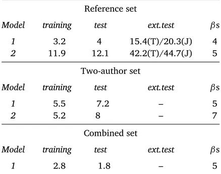
5.3 Comparison with previous results
(Klauss-Reference set
Model training test ext.test βs
1 3.2 4 15.4(T)/20.3(J) 4
2 11.9 12.1 42.2(T)/44.7(J) 5
Two-author set
Model training test ext.test βs
1 5.5 7.2 – 5
2 5.2 8 – 7
Combined set
Model training test ext.test βs
[image:25.482.59.278.69.242.2]1 2.8 1.8 – 5
Table 6:
Results for previous work (Klaussner and Vogel 2015), showing RMSE and model size for the reference corpus, the James and Twain data set, and the combination of all three data sets
fea-tures change in frequency over time, and how those changes are to be interpreted. The latter task is open-ended, but depends on the former.
6
analysis of language change
In this section, we consider salient features of the regression models presented in Section 5.2. In order to select those features that change most over time, we rank the respective model’s predictors according to the absolute weight it is assigned in the model, thereby selecting features that increase and decrease linearly over time. However, to identify features that did not exhibit any change over time, we had to exclude features that rated high on either linear or non-linear change. For this purpose, we evaluated all features separately with respect to the response variable, and selected those that rated low on both lin-ear and non-linlin-ear relationships. Section 6.1 introduces some general language change trends and Section 6.2 then analyses the data for the two authors in comparison with the reference corpus.
6.1 Reference language change
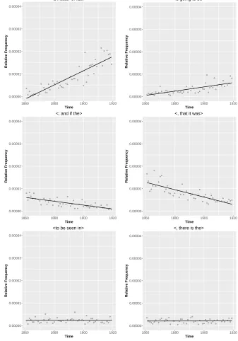
In the following, we present some aspects of general language change based on the changes detected in the reference corpus. This is not presented as an exhaustive list, but merely as a series of examples. In the following, we focus on lexical and syntactic change.
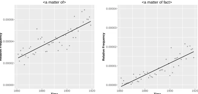
Figure 3 shows samples of the highest-rated features for each of the three categories: ‘increase over time’, ‘decrease over time’ and ‘no change’. Considering shorter n-gram sizes shows that there might be considerable overlap between different models of the same ture type but different n-gram size, and also between different fea-ture types. Figure 4 shows the word n-gram〈a matter of fact〉 and its hypergram〈a matter of〉. As can be seen from the difference in fre-quency, there are a number of other frequent realizations of〈a matter of〉, such as 〈a matter of concern〉 or 〈a matter of urgency〉. There are cases where the more specific sequence accounts for most of the occurrences of the generic one, whereas in cases like these it only ac-counts for part of them.
● ● ● ●● ● ● ● ● ● ● ● ● ● ● ● ● ● ● ● ●● ● ● ● ●● ● ● ● ● ● ● ● ● ● ●● ● ● ● ● ● ●● ●● ● 0.00000 0.00001 0.00002 0.00003 0.00004
1860 1880 1900 1920
Time
Relative Frequenc
y
<a matter of fact>
● ●● ●● ● ●● ● ● ● ● ● ●● ● ● ● ● ●●● ● ● ● ● ● ●● ● ● ● ● ● ● ● ● ● ● ● ● ● ● ● ● ● ● ● 0.00000 0.00001 0.00002 0.00003 0.00004
1860 1880 1900 1920
Time
Relative Frequenc
y
<is going to be>
● ● ● ● ● ● ● ● ● ● ● ● ● ● ● ● ● ● ● ● ● ●● ● ● ● ● ●● ● ● ● ● ● ●● ● ●● ● ● ● ● ● ● ●●● 0.00000 0.00001 0.00002 0.00003 0.00004
1860 1880 1900 1920
Time
Relative Frequenc
y
<; and if the>
● ● ● ● ● ● ● ● ●● ● ● ● ● ● ● ● ● ● ● ● ● ● ● ● ● ● ● ● ● ● ● ● ● ● ● ● ● ● ● ● ● ● ●● ●●● 0.00000 0.00001 0.00002 0.00003 0.00004
1860 1880 1900 1920
Time
Relative Frequenc
y
<, that it was>
● ● ● ● ● ● ● ● ● ● ● ● ● ●● ● ● ● ●● ●● ● ●●●● ● ● ●●● ● ● ● ● ● ● ●● ● ● ● ● ● ● ● ● 0.00000 0.00001 0.00002 0.00003 0.00004
1860 1880 1900 1920
Time
Relative Frequenc
y
<to be seen in>
● ● ● ● ● ● ● ● ●● ● ● ● ● ● ● ● ● ● ● ● ● ● ● ●● ●● ● ● ● ● ● ● ● ● ● ● ● ● ● ● ● ● ● ● ● ● 0.00000 0.00001 0.00002 0.00003 0.00004
1860 1880 1900 1920
Time
Relative Frequenc
y
[image:27.482.56.393.75.557.2]<, there is the>
● ● ● ● ● ● ● ● ● ● ●● ● ● ●● ● ● ● ● ● ● ● ● ● ● ● ● ● ●● ● ● ● ● ● ● ● ● ● ● ● ● ● ● ● ● ● 0.00000 0.00002 0.00004 0.00006
1860 1880 1900 1920
Time
Relative Frequenc
y
<a matter of>
● ● ● ●● ● ● ● ● ● ● ● ● ● ● ● ● ● ● ● ●● ● ● ● ●● ● ● ● ● ● ● ● ● ● ●● ● ● ● ● ● ●● ●● ● 0.00000 0.00001 0.00002 0.00003 0.00004
1860 1880 1900 1920
Time
Relative Frequenc
y
[image:28.482.92.420.69.226.2]<a matter of fact>
Figure 4: Reference corpus: relative frequency for〈a matter of〉 and〈a matter of fact〉
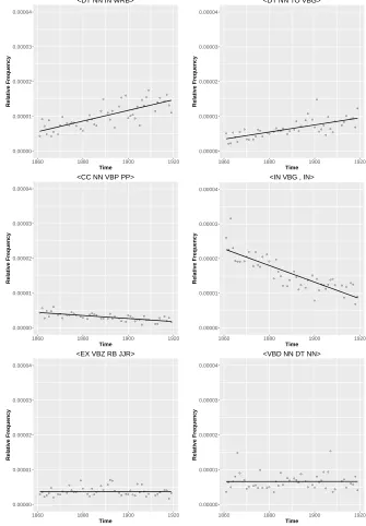
time. Phrases such as 〈the fact that when〉 or〈the secret of where〉 are examples of the former, and〈no objection to saying/taking〉 or〈a view to showing/discovering〉 are examples of the latter. Thus, de-pending on whether the words in the sequence are content or function words, and whether they are part of a collocation, certain combina-tions will be more frequent (〈a view to〉/〈no objection to〉), while others may be more variable. The shorter variant of this 〈DT NN TO〉 does not seem to be discriminative over time. Similarly, exam-ining some corresponding syntactic word sequences 〈a.DT view.NN to.TO〉 and 〈no.DT objection.NN to.TO〉 shows that, although con-stant, they do appear to change in a rather random fashion. The more specific tetragram sequences, such as 〈no objection to saying〉 are usually not constant. Realizations of decreasing POS features (〈CC NN VBP PP〉 and 〈IN VBG , IN〉), also yield patterns of fixed and varying units: 〈and pride/happiness attend her〉 and 〈by saying, that〉/〈without murmuring, because〉. The syntactic combinations that show the least development during this time span are〈EX VBZ RB JJR〉 with examples such as 〈there is far more/less〉/〈there’s some-thing stronger〉, and〈VBD NN DT NN〉with examples like〈was noth-ing the matter〉 or〈made music all day〉.
us-● ● ● ● ● ● ● ● ● ● ● ● ● ● ● ● ● ● ● ● ● ● ● ● ● ● ● ● ● ● ● ● ●● ● ● ● ● ● ● ● ● ● ● ● ● ● ● 0.00000 0.00001 0.00002 0.00003 0.00004
1860 1880 1900 1920
Time
Relative Frequenc
y
<DT NN IN WRB>
● ● ● ● ● ● ● ● ● ●● ● ●● ● ●●● ● ● ● ● ● ●● ● ● ● ● ● ● ● ● ● ● ● ● ● ● ● ● ● ● ● ● ● ● ● 0.00000 0.00001 0.00002 0.00003 0.00004
1860 1880 1900 1920
Time
Relative Frequenc
y
<DT NN TO VBG>
● ● ● ● ● ● ● ●● ● ● ● ● ● ● ● ●● ●● ● ● ● ●● ● ● ● ● ●● ● ● ● ●● ● ● ● ● ● ● ● ●● ● ● ● 0.00000 0.00001 0.00002 0.00003 0.00004
1860 1880 1900 1920
Time
Relative Frequenc
y
<CC NN VBP PP>
● ● ● ● ● ● ●● ● ● ● ● ● ● ● ● ● ● ● ● ● ●● ● ● ● ● ● ● ● ● ● ● ● ● ● ● ● ● ● ● ● ● ● ● ● ● ● 0.00000 0.00001 0.00002 0.00003 0.00004
1860 1880 1900 1920
Time
Relative Frequenc
y
<IN VBG , IN>
● ● ●●● ● ● ● ● ● ● ● ● ● ● ● ● ● ● ● ● ● ● ● ● ● ● ● ● ●● ● ● ●● ● ● ● ● ● ● ●● ●● ● ● ● 0.00000 0.00001 0.00002 0.00003 0.00004
1860 1880 1900 1920
Time
Relative Frequenc
y
<EX VBZ RB JJR>
● ● ● ● ● ● ● ● ● ●● ● ● ● ●● ● ● ● ● ● ● ● ● ● ● ● ● ● ● ● ● ● ●● ● ● ● ● ● ● ●● ● ● ● ● ● 0.00000 0.00001 0.00002 0.00003 0.00004
1860 1880 1900 1920
Time
Relative Frequenc
y
[image:29.482.57.392.73.555.2]<VBD NN DT NN>
age found in these genres. In spite of this, most of the consistent features or their generalizations present here seem to be expressing opinions, or to be ways of organizing these, such as 〈a matter of fact〉 or 〈a view to〉/〈no objection to〉, which are items that could be expected to appear in a variety of contexts. In order to identify change that is not general to all written language, one might inves-tigate change in different genres, such as fiction, or newspaper arti-cles. The most dramatic change is found in very general POS n-grams, which incidentally also display more spread. In contrast to syntactic word n-grams, POS n-grams are more volatile in that they represent a group of words that could possibly change or give rise to different frequencies.
6.2 Two-author language change
We now turn to the analysis of the two authors, to examine how their language changed or stayed the same over time, while also taking into consideration how their language differed from the reference language of the time. In the following, we consider different aspects of how style could vary. Section 6.2.1 considers differences between constant feature sets of lexical types. Sections 6.2.2 and 6.2.3 consider stylistic differences between the reference corpus and the two authors, and then any stylistic differences between the two authors.
6.2.1 Constant features
In order to explore the stylistic differences between Mark Twain and Henry James, we examine different sets of constant terms: those they share and those they do not share. It is important to note that con-stancy does not necessarily imply high frequency, and that one word or expression could be constant for only one author but more frequent overall for the other.
Figure 6 shows ‘wordclouds’ based on their individual non-shared noun, interrogative pronoun, and adjective type features. We grouped these together for inspection since they could all occur in noun phrases but, unlike pronouns and determiners, are less grammatically con-trolled, and therefore more meaningful.
Figure 6: Noun, interrogative pronoun, and adjective type wordclouds for Twain (left) and James (right), based on non-shared constant features
Twain’s most prominent words express existential concepts, ap-parently pertaining to a more questioning nature, e.g. ‘god’, ‘money’, ‘ everybody’, ‘anybody’, ‘nobody’, ‘family’, ‘mother’, ‘children’, ‘dead’, ‘heaven’, ‘church’, ‘trial’, and ‘soul’. In contrast, James’ most promi-nent words in this group are more prosaic, e.g. ‘mr’, ‘father’, ‘lady’, ‘dear’, ‘whom’, ‘lord’, ‘charming’, ‘companion’, ‘impression’.30 It is interesting to note the difference between James’ most frequently used form of address, ‘Mr’, and Twain’s ‘Sir’ – ‘Mr’ suggests that one could address both a superior and an equal, whereas ‘Sir’ is used pre-dominantly when addressing a superior, which is plausible as Twain also wrote about less wealthy people.31 James’ list also includes the French word ‘de’, often found in names and addresses and, which was incorrectly tagged here as a proper noun.32 There are some other interesting contrasts, such as ‘conscience’, which is constant for Twain, and ‘conscious’/‘consciousness’, constant for James. Twain’s words suggest more intense situations, intimating both good and bad, e.g. ‘crime’, ‘cruel’, ‘blood’, ‘dark’, ‘lonely’, ‘alive’, ‘peace’. James’ most negative words in this group are ‘sad’, ‘helpless’, ‘victim’, indicating that Twain’s language was more explicit. While James’ stories do con-tain conflicts, they were possibly more veiled than in Twain’s texts.
30As all data was transformed to lowercase for analysis, words, such as ‘Mr’ appear that way in figures as well.
31The word ‘Sir’ is ranked 19 among wordcloud features and 381 among Twain’s constant features.
Figure 7: Noun and adjective wordclouds for Twain (left) and James (right), based on their shared constant features
Figure 7 shows the wordclouds for their shared constant nouns, interrogative pronouns, and adjectives. Their most prominent words are quite similar here, e.g. ‘what’, ‘time’, ‘little’, ‘good’, and ‘young’. There are some less frequent words for both that are interesting to con-sider, with a wider semantic range: ‘circumstances’, ‘feeling’, ‘conse-quence’, ‘believe’, ‘truth’, and ‘pleasure’. Depending on context, these words might take on either a more superficial or deeper meaning, e.g. ‘I believe you’re right’ and ‘I believe in one Christ’.
Interestingly, both authors took an avid interest in history, evi-denced by the syntactic unigram〈history〉 being among their shared constant features. Both Blair (1963) and Thomas M. Walsh and Thomas D. Zlatic (1981) note that history played an important part in Twain’s personal as well as his professional life, even if he did not al-ways incorporate his knowledge consistently into his works (Williams 1965). In his 1884 essay ‘The Art of Fiction’, James actually claims his place among historians, since a novelist chronicles life, and as ‘picture is reality, so the novel is history’ (James 1884). All of the two authors’ constant word unigrams are present in the constant features of the reference corpus, except for James’ term ‘vagueness’.33
While constant word unigrams reveal a great deal about recur-ring concepts, longer sequences might hold more information about unique aspects of style, as these tend to be more generic. Table 8 shows examples of constant bigram and trigram word sequences and
their frequencies found in the data for Twain, for James, and for Twain and James together. These lists are mutually exclusive, meaning that each term is shown only once, in the set where it is most constantly used. The rows group together n-grams by selection category. The first group contains bigram sequences of a noun followed by a preposition followed by either a male or female possessive pronoun. The second group contains singular or plural body references, either followed by a comma, or preceded by a male or female possessive pronoun. The third group contains expressions that are used for emphasis or con-trast. The last two groups focus on items expressing some epistemic commitment, or with an existential construction.
Twain’s language, in particular, abounds with a great variety of body references, some of which are also used by James. How-ever, James tends to focus on body descriptions, e.g. ‘face’, ‘eyes’, ‘hands’, whereas Twain’s constant terms include items used more ab-stractly, such as ‘heart’. Twain’s language also features many more ‘existential’ constructions, such as 〈there ’s〉, which are also found in James, but with less variety. Both authors use expressions in-dicating reflection or thought (〈I know〉, 〈I think〉, etc.). Twain’s constant terms also include the expression 〈don’t know〉, which James does not appear to use. James seems to use contrasting fea-tures more often, e.g. 〈in spite of〉 or 〈, however ,〉, which Twain appears to employ more sparingly. Both use the male perspective more than the female one, i.e. their constant feature lists both con-tain various possessive and regular pronoun constructions for male characters, which are not present in the same quantity for female characters.
Figure 8: Existential〈there〉
for all three corpora
●
●●
● ●
●
●● ● ●
● ● ● ●
● ●
● ● ● ●
● ●
●
● ●● ●●
● ●
●● ●
●● ●
● ● ● ● ● ●
● ●
● ●
● ●
● ●● ● ●
●● ●●
● ●
0.0010 0.0015 0.0020 0.0025
1860 1870 1880 1890 1900 1910 Time
Relativ
e Frequency
● RC
Twain
James
Table 9: Frequency and number of feature types for prominent constructions
James Twain Shared
Variable 1-gram:µ Lex2 Lex3 1-gram:µ Lex2 Lex3 Lex2 Lex3
〈there.EX〉 0.0018 3 – 0.002 7 4 4 2
body parts sing 0.0028 12 4 0.0029 14 2 4 –
body parts pl 0.001 1 – 0.001 5 1 3 –
female pr 0.023 8 1 0.008 20 5 17 –
male pr 0.025 9 2 0.025 49 54 27 9
them more often. There is also an increase in usage over time for both authors, as well as for the reference corpus.
Figure 9 depicts frequency rates for body references: Figures 9a and 9b show singular and plural body parts, respectively. Interest-ingly, average use for body references lies above the reference corpus for singular items and below it for plural items, in both Twain and James.34 There seems to be a decrease in usage for both types over time, with a more dramatic decrease for plural body parts. The differ-ence between the two authors lies primarily in the variety of construc-tions used: there tends to be more variety in Twain’s constant features – this does not mean that James does not use these features at all, but that there are fewer features that James uses regularly.
● ●
● ●●● ●●
●
● ● ● ●
● ●
●●● ●
● ●● ●
● ●
● ●
● ●
● ● ●
● ●● ●
● ●● ●
● ●
● ● ●
● ●
● ● ●
● ●●
● ●
● ●
● ●
0.000 0.001 0.002 0.003 0.004
1860 1870 1880 1890 1900 1910
Time
Relativ
e Frequency
● RC
Twain
James
(a) Frequency of singular body parts for James, Twain, and the RC
● ● ●● ● ● ●
●●● ● ● ●
● ●
● ● ●●● ● ● ● ●
● ●
● ● ●
● ●
● ●● ● ●●●● ●
● ●
●
● ●● ●● ●● ●● ● ●● ● ●
● ●
0.000 0.001 0.002 0.003 0.004
1860 1870 1880 1890 1900 1910
Time
Relativ
e Frequency
● RC
Twain
James
(b) Frequency of plural body parts for James, Twain, and the RC
[image:37.482.61.370.272.454.2]Figure 9: Body part constructions for all three corpora
Figure 10: Male and female references for all three corpora
●● ●
●● ● ●● ●
● ●
● ● ●
● ●
● ●
● ● ● ●
●
● ●● ● ●● ●● ●
●● ● ●● ●● ●
● ●
● ●●
●
●● ● ●● ●●●● ●
● ● ●
0.00 0.01 0.02 0.03 0.04
1860 1870 1880 1890 1900 1910 Time
Relativ
e Frequency
● RC
Twain
James
(a) Frequency of male pronouns for James, Twain, and the RC
● ●
● ● ●
● ●● ● ●
● ●
● ●
●
● ●
● ●●●
● ●
●
● ●
● ●
● ●● ● ●● ● ●
●●● ●
● ●
● ● ● ● ●
● ● ●
● ●
● ●
●● ● ● ●
0.00 0.01 0.02 0.03 0.04
1860 1870 1880 1890 1900 1910 Time
Relativ
e Frequency
● RC
Twain
James
(b) Frequency of female pronouns for James, Twain, and the RC
contem-poraneous authors, to examine the proportion of gendered pronoun constructions in their non-constant bigrams, it is not clear whether this aspect is usual or unusual. For instance, James might only have a few constant constructions, changing his language use depending on the situation.
6.2.2 Stylistic differences with the reference set
In order to explore any differences from the reference language, we consider the shared salient features, i.e. the features that appear in Twain, in James, and in the reference corpus. Among the charac-ter n-gram models, there are no common predictors, except for the letter 〈q〉 in the unigram model. All models have a positive weight for this predictor, but only the authors show a clear upward trend over time. All word stem and syntactic word n-gram models yield one shared bigram 〈, by〉, which is shown in Figure 11 and Figure 12, together with three highly weighted shared POS bigrams 〈CC EX〉, 〈WDT ,〉 and〈MD ,〉.
The bigram〈CC EX〉 realizes expressions such as〈but there〉 or 〈and there〉, that have already been mentioned earlier with respect to the constant features in James and Twain. For this POS bigram, their average rate tends to be higher than that of the reference corpus. What is noticeable for the other three features is that the three data sets are rather well separated, with James having the highest usage of all. This will be explored in more depth as part of the between-author analysis in Section 6.2.3. All lines show some development over time, explaining why these are salient features in the models.
Figure 11: Prominent features common to Twain, James, and the reference corpus
●
● ●
● ●
●
●● ● ●● ● ● ●●
● ● ● ● ●
● ●
● ●
● ● ● ● ● ● ●
● ●
● ●●● ● ● ● ● ●
● ●
●● ●
●
● ● ● ● ● ● ● ● ● ●
●
0.0000 0.0001 0.0002 0.0003 0.0004 0.0005
1860 1870 1880 1890 1900 1910 Time
Relativ
e Frequency
● RC
Twain
James
(a) Frequency of〈CC EX〉 for James, Twain, and the RC
● ● ●
●
● ● ●●
●
● ●●
● ●
● ●
● ●● ●● ●
● ●●● ● ● ●
● ●
● ● ● ● ●●● ● ●●
● ●
● ● ●●● ● ● ● ● ● ● ● ● ● ●●
0.00000 0.00025 0.00050 0.00075 0.00100
1860 1870 1880 1890 1900 1910 Time
Relativ
e Frequency
● RC
Twain
James
(b) Frequency of〈, by〉for James, Twain, and the RC
● ●
● ● ● ●
●● ●
●● ●●● ●
● ● ●●●●
● ●●
● ● ● ●● ●● ● ●● ● ●● ● ●●● ●
● ● ●
●
● ● ● ● ● ●●● ● ● ●● ●
0.00000 0.00025 0.00050 0.00075 0.00100
1860 1870 1880 1890 1900 1910 Time
Relativ
e Frequency
● RC
Twain
James
(a) Frequency of〈WDT ,〉for James, Twain, and the RC
● ●
● ●
● ●
●● ●
● ●
● ●●
● ●
● ● ● ● ●●
● ● ●
● ●
● ●
● ●
● ●● ● ●●
● ●
● ● ● ●●
●● ● ●
●● ●
● ● ●
● ●
● ●
●
0.0000 0.0001 0.0002 0.0003 0.0004 0.0005
1860 1870 1880 1890 1900 1910 Time
Relativ
e Frequency
● RC
Twain
James
(b) Frequency of〈MD ,〉for James, Twain, and the RC
Figure 12: Prominent features common to Twain, James, and the
reference corpus
6.2.3 Stylistic differences between authors