Priority based Energy Efficient Dynamic Power Scaling

ABSTRACT

As part of the energy efficient system modeling, which is of interest amongst all areas of research in industry and academia, this paper proposes a design of energy efficient Ethernet access system. The model estimates the feasibility of operating the network interface component under power saving modes, without compromising on the quality of service. In order to prevent degradation of the service quality, the constraint ensures that the estimated duration of sleep time does not go beyond a certain threshold parameter, or maximum allowable delay limit per packet processed, within a given flow. The allowable limit or threshold value of the delay is fixed across each flow and corresponds to its priority tag, where a higher priority means, lower allowable delay. Simulations have been carried out for the algorithm and graphs plotted, to validate the feasibility of the proposed model.

Index Terms— Energy Efficient Systems, Access Networks, Exponential Smoothing, Active and Sleep State

1. INTRODUCTION

The global CO2 emissions due to ICT equipment alone is

estimated to be 2% worldwide and is expected to grow to 4% by 2020 as recent studies have suggested [2-3]. ICT has traditionally enjoyed the reputation of being a green technology as is obvious with the infrastructure supporting voice and video conferences, online meeting and training facilities, which saves considerable energy in commuting across locations and hence has a positive impact on the environment and nature. But with the massive growth of internet and ubiquitous nature of internet enabled devices, has raised the concerns of energy consumption in the ICT sector. Energy efficient system design and dynamic power scaling has been the interest of researchers across all fields. A part of the current research focuses on enabling energy saving techniques across the underutilized customer premise access equipment’s. A pre calculated and coordinated decision of low power states, based on arrival pattern can lead to considerable power savings when aggregated over a period of time. While the decision of enabling energy efficient modes is of important, simultaneously the algorithm needs to ensure that degradation in service quality due to additional delay is kept to minimal.

2. BACKGROUND STUDY

Research done by Christensen et al. [9-10] has led to the standardization of the IEEE 802.3az Ethernet standard, which defines the low power idle state and the active modes of operation, with a refresh timer to keep the current status of the system synchronized.

Between power management and performance, there exists an inherent conflict as it is understood, that the more power that is available to a system, the better is its

performance. So, during the times that performance is less critical, power management techniques can be applied. And that essentially means, a suitable technique must be in place which decides the performance requirements of a system at any point in time and hence applying the appropriate power reduction technique.

Yao et al. [4] have proposed an optimization problem, where the objective is to minimize the energy consumption based on the deadline feasibility. The algorithm proceeds through a series of iterations, and in each interval the tasks are scheduled based upon earliest deadline first, within the limitations of the intensity interval. The intensity of the interval is the sum of the work times of all the tasks.

Any scheduling problem can be considered parallel as a energy management or a temperature management problem. The model is based on a dual optimization problem, where the objectives are quality of service and energy or temperature minimization. In [15] the authors have proposed the introduction of energy-awareness into control plane protocols whose goal is to properly condition all the route/light path selection mechanisms on relatively coarse time scales by privileging the use of renewable energy sources and ether efficient links/switching devices. By combining, the notable features that a comprehensive energy aware network model should have and put them into a constrained routing and wavelength assignment problem framework.

The ILP formulation while effective in its formulation and descriptive power is inherently static and hence implies a-priori knowledge of the entire traffic matrix to be solved at optimum. The objective is to route the requested light paths so that the overall network GHG emissions are minimized.

Dhiman et al. [16] have proposed a mechanism of dynamic power management using machine learning. Dynamic power management relies on the policy of selective shutdown of the system components when idle in order to reduce the power dissipation. The policy must ensure that the power savings options are maximized while the performance degradation and delay are kept within acceptable limits.

The simpler policies do it heuristically, while complex ones guarantee optimality for stationary workloads. The authors have proposed a control mechanism, where the algorithm selects the best suited dynamic power management policy from amongst a given set. So, given an idle period, the controller needs to ensure that a DPM policy is selected from amongst, (i) fixed, or (ii) exponential predictive, or, (iii) stochastic policies.

The set of experts is referred to as the working set, and the selected expert is the 'operational' one and rest is dormant for the given workload. The algorithm performs machine learning, to select the expert with the highest probability of performing well, under the given circumstances. The algorithm associates and maintains a weight vector which associates the experts to their weights and a higher weight indicating a better performance. In [17] the author has proposed an energy delay product for

Priority based Energy Efficient Dynamic

Power Scaling

Rakesh Kumar Pradhan

Mark A Gregory

energy efficient design. The energy delay product is to be optimized by fixing one and minimizing the other. In his paper, two approaches are recommended - (i) Observing the energy conservation constraint, and fixing the schedule length, which has got applications in multiprocessor systems, where energy conservation is an important concern, (ii) with schedule length (delay) as a constraint minimizing the energy consumption, which has got applications in real time systems, where timing plays a critical role.

The system partitioning, power supplying and the schedule length has to be divided as three separate tasks that needs to be dealt with separately. The problem can be formulated as; given a set of n tasks, t1, t2, … tn with the delay requirements as d1, d2, d3,

... dn the task is to find the power supplies p1, p2, p3, … pm in a m

processor multitasking environment such that, the energy consumption is minimized. The same needs to be done under the constraint that the cumulative delay requirements do not exceed, T.

Singh et al. [6] have considered how the architecture of the internet can be modified to ensure energy efficiency. The basic principle is, when some of the components are idle the hardware can be clocked slower or some of the components can be switched off (ex- network interface card). At the network level, some of the routes can be re-modified, or aggregated, during the periods of low activity to ensure that only the busy routes are operational and the idle routes are put to sleep modes, in order to ensure power conservations. At the internet topology level, route adaptation can ensure that during periods of activity and inactivity, and based on the load, some or more of the components in a cluster can be put to sleep, based on more route selection options.

3. EVALUATION METHODOLOGY

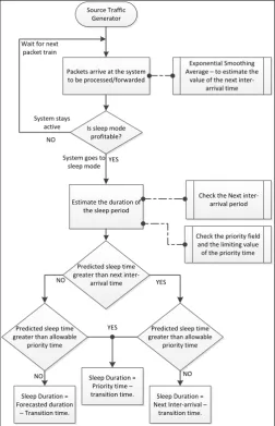
As part of the simulation, packets are generated from the source node, of fixed size, and random exponentially varying inter-arrival times. The random nature of the inter-inter-arrival times are generated via discrete event C++ simulation, and the events stored in the form of an array. The number of packets is varied for generating different plots as shown in the graphs below. Based on the arrival pattern of the incoming traffic, an estimate is done of the next inter-arrival duration using exponential smoothing forecasting method, which smoothens the predicted duration as per the current arrival and past history. It uses a fixed weight factor also called as smoothing constant.

Based on the current prediction, the algorithm decides, whether it is feasible to put the system under consideration into low power or sleep states. If the decision status is positive, the algorithm compares the forecasted duration of the sleep time with the prioritized traffic, maximum allowable delay.

Source Traffic Generator

Packets arrive at the system to be processed/forwarded

Exponential Smoothing Average – to estimate the

value of the next inter-arrival time

Is sleep mode profitable?

Estimate the duration of the sleep period NO

Wait for next packet train

YES

Check the Next inter-arrival period System stays

active

System goes to sleep mode

Check the priority field and the limiting value of the priority time

Predicted sleep time greater than next

inter-arrival time

Predicted sleep time greater than allowable

priority time Predicted sleep time

greater than allowable priority time

YES NO

Sleep Duration = Priority time – transition time.

YES

Sleep Duration = Forecasted duration

– Transition time.

Sleep Duration = Next Inter-arrival –

transition time.

NO NO

Fig 1. Algorithm decision flow

The priority tag is corresponding to an individual flow and puts a limiting value on the duration of the sleep time for every processed packet. If the estimated value of the sleep duration falls below the maximum allowable delay, then the system sleeps for the forecasted duration of time, keeping the transition time into consideration. When the estimated sleep duration exceeds the prioritized maximum allowable delay, then the sleep time is reduced to the limiting value of delay, keeping transition time into account. In case of a non-profitable value of the sleep duration, the system continues to operate in the active region without any transition to low power states.

A. Exponential Smoothing Average

An exponential smoothing average is used to forecast the next inter-arrival time duration. The forecast value is computed from the current actual value of the inter-arrival time and the previous forecast value as shown in (1).

Ft+1 = (Actual Value*α) + (1–α)*(Previous forecast)

(1)

Where, α is the exponential smoothing weight and has a value 0 < α < 1. For the simulation model presented in this paper, the value of α was set to 0.125. The choice of α was based on [6].

B. Transition Period Calculation

In order to be able to save power by putting the system into sleep mode, it is important to ensure that the sum of the power consumption during the sleep state and the transition (low – high) is less than the equivalent power consumed if the system were to remain in the active state as shown in (2).

((Sth - )*Es + *Ew ) < Sth*Ei

(2)

Where, Sthis the threshold period for the decision to move to

sleep mode. is the transition time taken to move from the

sleep mode to the active state. Es, Ew, Eiare the system power consumption during the sleep, transition and active states respectively.

So, (2) results in the inequality shown in (3).

Sth  (Ew – Es)(Ei – Es)

(3)

C. Energy Consumption Equations

The total power consumed is the sum of the power consumed during the sleep state and the state transitions as shown in (4).

Esleep = EsTs + Ei(T – NTp – Ns - Ts) + NsEw

(4)

The values of Ns and Ts are calculated from the algorithm.

Other values as Es, Ew, Ei,  and T are system inputs. The total

power consumed during the active states is the sum of the power consumed in the active state and the cumulative power needed to transmit all of the packets.

Eactive = Ei (T – NTp) + NEpTp

(5)

The parameters used for the purposes of simulation are; Ei

(active state power) = 1W, Ep (power for processing a packet) =

2W, Ew (power during transit - low to high) = 2W, and Es (sleep

state power) = 0.1W. During the simulations the packet processing time Tp was set to 0.00012s (1500 MB packet at a 100

Mbps interface, time for processing a packet is 0.00012s (1500 * 8 / (100 * 10^6)).

4. RESULTS AND DISCUSSION

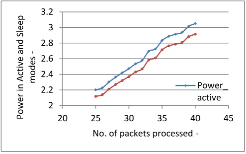
Fig. 2 shows the Energy consumption values with varying number of packets processed. The simulation was carried out by increasing the number of packets processed (and hence inter-arrivals) from 25 to 40, by steps of 1. The resultant power saving was also observed to increase with the increase in the number of packets processed. The Total energy consumption in the active state with 25 packets processed was 2.2001 W and in the sleep state was found to be 2.11611. The effective power savings was 0.084. The total energy consumption during the active state, with 40 packets processed was found to be 3.05091, and the corresponding energy consumption with the sleep modes is 2.91441. The difference between the same and hence the effective power savings was 0.1365W.

Fig 2. Power consumption v/s no. of packets processed.

Hence the energy difference was observed to increase from 0.084 to 0.1365 with the number of packets processed increasing from 25 to 40. The rise in the power savings can be attributed to the fact that, with the growth in the inter-arrival there is also a rise in the frequency of sleep or active states. So, with the increase in the number of sleep states, with each of these inter-arrivals, the aggregated duration of sleep time also increases, and hence these is an increase in the energy savings as per the simulation results.

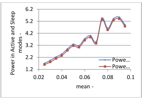
Fig. 3 displays the simulation results of the varying mean which is required for generating the exponential random inter-arrival periods, versus the calculated power consumption in the active and sleep states.

The energy consumption within the active and the sleep states are both found to be on the rise, with the increase of the mean value, with an almost constant difference. The mean values were varied from 0.025 till 0.095 with a step increase of 0.005. The energy consumed with the mean value of 0.025 was found to be 1.69922 W in the active state and the corresponding valuw in the sleep state was found to be 1.58975. The effective energy savings for the same was calculated to be 0.10947. The highest value of the mean was 0.095, in the simulation parameters and the correspongin energy consumption values in the active and sleep states was found to be 4.90602 and 4.76952, which calculates to an energy differential of 0.1365.

2 2.2 2.4 2.6 2.8 3 3.2

20 25 30 35 40 45

Po

w

er

in

Act

iv

e

an

d

Sle

ep

m

o

d

es

Fig 3. Power consumption v/s mean inter-arrival time.

Variations are observed within the active and sleep states, as seen in the graph. While there is a peak of the power consumption values (in both states) for a mean value of 0.075, the same undergoes a drop and increase again, with the changing values of the mean value for inter-arrival. The same is attributed to the fact that, while a rise in inter-arrival mean could imply increased number of the sleep and active states, however with the limiting value of the priority time, set to 0.025s (or 25 ms), there is a cap on the duration for which the device can be operational within the sleep and active states. And so, based on the random value of the actual and forecasted inter-arrival period and the limiting value of the priority time, the power consumption within the active and sleep states is found to be varying.

Fig. 4 shows the power consumed during the active and sleep modes with a varying number of packets processed. As the number of packets processed increases, the energy consumed in both the active and sleep modes increases.

For the simulations the number of packets processed was varied from 30 to 50 incrementing by steps of 2. In 60% of the cases, the power consumed in the sleep mode was found to be less and hence resulting in power savings. In some circumstances the power consumed in the sleep mode exceeded the power consumed during the active mode, due to the increase in the number of transitions as the number of packets processed was increased. The power consumed in the active mode was found to be 3.01982W, for 30 packets, and increased to 3.78159W for 48 packets processed. The value of the power consumed during the sleep mode was found to be 2.88647W for 30 packets processed and increased to 3.86232W for 48 packets processed.

Fig. 4 displays, the graphs plotted for the varying priority time versus the power consumption values in the active and the sleep states. The priority time is the limiting value of the duration of the sleep time, or the time period for which the system can be put into power saving mode. The priority time was varied from 0.025 s (25 ms) till 0.095 s in incremental steps of 0.005.

The total power consumption as calculated in the simulation during the active state for a priority time of 0.025 was found to be 3.05091 W and the corresponding value of power consumption in the sleep state was found to be 2.91441 W. The difference and the effective energy savings was observed to be 0.1365 W. The highest value of the priority time used within our simulation is 0.095 s (95 ms) and the values power consumption within the active and sleep modes are found to be 2.32896 W and 1.49674 W respectively. The maximum value of the active state

to be 1.36807 W for a limiting value of the priority time at 0.080 s.

Fig 4. Power consumption v/s priority allowable time.

Beyond the priority time of 0.055 S, the power consumption values for the sleep states are found to be normalizing across 1.5 W, with a maximum value of 1.69008 W and an observed minimum value of 1.36807 W. The maximum energy savings was found to be 1.7395 for a priority limiting value of 0.075 s.

5. CONCLUSION

This paper presents analysis of energy efficient characteristics in an Ethernet access network. Simulations have been carried out with given input parameters (as specified) and results display a distinct advantage towards power saving modes of operation, under low load conditions, with fixed quality of service delay constraints. The quality of service factor indicates a maximum allowable delay per processed packet. Statistics have been collected for various values of maximum allowable delay as per the priority tag. Graphs have been plotted based on event driven simulation for the same. As part of future research, we plan to include buffer as the additional parameter for effective power savings. The inclusion of buffer will enable the differential rates of arrival and service rates to be exploited on a case by case basis and allow additional power savings modes to be introduced. The segregation of the power saving modes based on selective component operations (on/off states) will provide an extra dimension in design of network architecture.

REFERENCES

[1] C. H. Hwang and A. C. H. Wu, "A predictive system shutdown method for energy saving of event-driven computation," ACM Transactions on Design Automation of Electronic Systems (TODAES), vol. 5, pp. 226-241, 2000.

[2] S. Evans and J. Millen, "ICT's Role in the Low Carbon Economy," Australia Information Industry Association, Australia, September 2010.

[3] M. Webb, "Smart 2020: Enabling the low carbon economy in the information age," The Climate Group London, 2008.

[4] F. Yao, A. Demers, S. Shenker, “A scheduling model for reduced CPU energy”, IEEE, 1995, 374-382.

[5] S. Irani, S. Shukla, R. Gupta, “Algorithms for power savings”, Society for Industrial and Applied Mathematics,

1.2 2.2 3.2 4.2 5.2 6.2

0.02 0.04 0.06 0.08 0.1

Po

w

er

in

Act

iv

e

an

d

Sle

ep

m

o

d

es

mean -

Powe… Powe…

1 1.5 2 2.5 3 3.5

0.02 0.04 0.06 0.08 0.1

Po

w

er

in

Act

iv

e

an

d

Sle

ep

m

o

d

es

priority time - Power_

[6] M. Gupta, S. Grover, S. Singh, “A feasibility study for power management in LAN switches”, IEEE, 2004, 361-371.

[7] M. Gupta and S. Singh, "Greening of the Internet," 2003, pp. 19-26.

[8] M. Gupta, S. Singh,” Dynamic ethernet link shutdown for energy conservation on ethernet links”, IEEE, 2007, 6156-6161.

[9] K. Christensen, et al., "IEEE 802.3 az: the road to energy efficient ethernet," Communications Magazine, IEEE, vol. 48, pp. 50-56, 2010

[10]C. Gunaratne, et al., "Reducing the energy consumption of Ethernet with adaptive link rate (ALR)," Computers, IEEE Transactions on, vol. 57, pp. 448-461, 2008.

[11]IEEE P802.3 az, "Energy Efficient Ethernet Task Force", 2010; http://grouper.ieee.org/groups/802/3/az/

[12]M. B. Srivastava, A.P. Chandrakasan, R.W. Brodersen, "Predictive system shutdown and other architectural techniques for energy efficient programmable computation," Very Large Scale Integration (VLSI) Systems, IEEE Transactions on, vol. 4, pp. 42-55, 1996.

[13]D. Ramanathan and R. Gupta, "System level online power management algorithms," IEEE, 2000, pp. 606-611.

[14]L. Cai, Y.H. Lu,” Dynamic power management using data buffers”, IEEE Computer Society, 2004, 10526.

[15]S. Ricciardi, et al., "Towards an energy-aware Internet: modeling a cross-layer optimization approach," Telecommunication Systems, pp. 1-22, 2011.

[16]G. Dhiman, T.S. Rosing, “Dynamic power management using machine learning”, ACM, 2006, 747-754.