A-Mazer with Genetic Algorithm
Nitin S. Choubey
Professor & Head, Computer Department MPSTME, SVKM’s NMIMS, Shirpur
Maharashtra, India-425405
ABSTRACT
Paper describes the approach of solving Maze problem with Genetic Algorithm. It also includes method for developing a rectangular maze structure, A-Mazer. The method is implemented and found to be effective for the maze structures with different complexity levels of the 20
20 size.
Keywords
Genetic Algorithm, Evolutionary Computation, Maze structure, Maze Complexity, NP-Complete.
1.
INTRODUCTION
For many real-world problems, the solution process consists of working your way through a sequence of decision points in which each choice leads you further along some path. Maze structures are also one of such problems. A maze is a grid-like two-dimensional area of any size, usually rectangular. A maze consists of cells. A cell is an elementary maze item, a formally bounded space, interpreted as a single site. The maze may contain different obstacles in any quantity. The complexity of the maze is determined by the number of cells, number of walls/obstacles, number of Hallways, dead-ends and the distance between the start-finish/Start-food cell in the maze structure [1].
[image:1.595.89.245.599.729.2]Mazes have been a part of human culture for thousands of years [2]
.
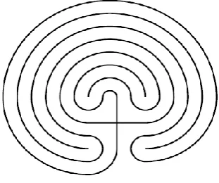
According to Greek Mythology, the Mediterranean island of Crete‟s king, Minos, created a maze referred as, labyrinth(See Fig. 1,) with the help of an engineering genius, Daedalus to house a deadly creature, Minotour. Young Theseus of Athens, entered the labyrinth with a sword and a ball of string. Theseus killed the Minotour and traced the path out of labyrinth by unwinding the string as he went along [3].
The term labyrinth is associated with the construction which leads from starting point to the goal state by taking tortuous path but requires no actual decision.Fig. 1. The Cretan labyrinth
Typically Mazes require sequence of decision to be taken in order to reach to the goal state from the initial state. The maze structure considered in this paper is a random rectangular maze constructed by using the sequence of stochastic decisions taken over iterations to create the same. The paper also focuses to give solution of the rectangular maze by using Genetic Algorithm, an evolutionary heuristic method for finding optimum solution.
Genetic algorithms are the heuristics methods from the category of evolutionary algorithms which are based on the Darwin‟s principle of origin of species by means of natural selection [4]. GA‟s are invented by John Holland in 1960‟s [5]. In contrast with Evolution Strategies and Evolutionary Programming, Holland‟s original goal was not to design algorithms to solve specific problems, but rather to formally study the phenomenon of adaptation as it occurs in nature and to develop ways in which the mechanisms of natural adaptation might be utilized into computer systems. Holland‟s 1975 book „Adaptation in Natural and Artificial Systems‟ presented the GA as an abstraction of biological evolution and gave a theoretical framework for adaptation under the GA. Many problems in engineering and related areas require the simultaneous genetic optimization of a number of, possibly competing, objectives have been solve by combining the multiple objectives in to single scalar by some linear combination[6].
Tremaux algorithm uses recursive backtracking procedure for finding the solution, which can be used to find path from inside the maze to the goal position outside the maze Dead End filling algorithm works well in the case when the maze have multiple dead ends but fails to get the optimum path when there exist more than one solution paths in the maze. A trivial method uses an unintelligent robot or a mouse which travels entire maze in random way. The method is referred as random maze solver and is a slow method to find the solution. There are several other methods such as Left wall follower, Use of Imaging, partition based maze solving but no specific method gives solution to the all the types of mazes[7][8].
Genetic algorithms are good heuristics which returns near to optimum solution. The objective of the paper is to provide a method to find path through maze using genetic algorithm. The method for generating the random rectangular maze structure with A-mazer and implementation details of the Genetic Algorithm used is given in Section 2. Experimental setup and the results are covered in Section 3 followed by concluding remarks in section 4.
2.
METHODOLOGY USED
2.1
A-Mazer
A-mazer is the technique used by the author for creation of maze structure. The maze structure is created by using the three step process described in the following subsections. It involves the creation of a random rectangular grid with size nn followed by assigning labels to the cells reachable from start and finish cells. If the labels assigned to the start and finish cell do not match the joining of the labels is done by the process of wall break down process.
2.1.1
Creation of the rectangular grid with
random door
It is the first step towards development of a random rectangular maze structure of size nn. The structure is a three-dimensional cube where each cell contains five elements representing availability of doors for the cell to the Left, Top, Right and Bottom boundary wall and the number of doors available in the current cell a shown below in fig 2.
Fig 2 : Data Structure used for storing the maze Fig 3.
The sample cell representation is shown in the inset. The doors are shown in Left and Bottom and the label is shown as „1‟.
The label is used in creation of the maze structure as well as for representing number of doors available in the cell during optimal path search process. Maze structure is updated by using procedure as shown in Fig. 3.
It returns „1‟ if there is path from Start cell to finish cell, otherwise it return „0‟ indicating non-availability of path.
2.1.2
. Labeling of the paths
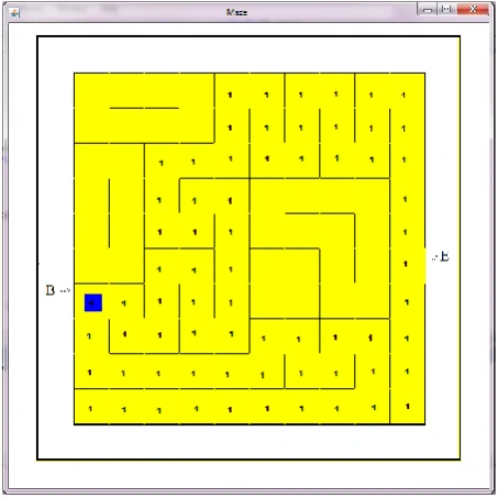
[image:2.595.52.279.260.516.2]The Start (S) and Finish (F) cells are randomly selected, 0 S, F n. The boundary is used for Start Cell and Right Boundary is selected for Finish cell. The cells are labels from the start node. The cell labeling is started with Start cell with label „1‟ by using Flood_Fill algorithm(S, 0) for every cell connected by door (Value = 1) [9]. If the labeling is done to Finish cell (0, F) also, Return(1), Otherwise Use Flood_Fill(F,n) with label „2‟. Fig 4 shows the case of Return(1).
Fig. 3. Creation of Random Maze Structure
In the case of Return Value as a 0, the process of join the Labels is adopted to create the maze.
2.1.3
Join the labels
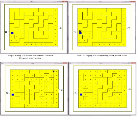
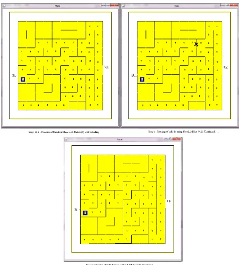
[image:2.595.316.543.516.743.2]In this process, the tracking of the label is done by using flood_fill algorithm for the walls exist between cells. If a wall is in between the cells with different labels and one of the label is „1‟, it is merge in to the cell with Label value = „1‟. The process is continued till the cell with Label Value =‟2‟ is merged in to the cell with Label value = „1‟. The process for joining the labels is shown in fig 7 & 8.
Fig 4. Case of Valid Random Maze
1. Create an nn structure, Maze M, containing five cells for indicating Left, Top, Right and Bottom doors with door value „0‟ for walls.
2. Repeat step 3 for all cells M(i,j), except boundary cells. 3. Repeat steps for each value of Left, Top, Right, and
bottom. a. Left :
i. Generate random number n(0,1)
ii. If(n==1), assign Left =1 (Create Door) & Right = 1 in the cell (i,j-1).
b. Right :
i. Generate random number n(0,1)
ii. If(n==1), assign Right =1 (Create Door) & Left = 1 in the cell (i,j+1).
c. Top :
i. Generate random number n(0,1)
ii. If(n==1), assign Top =1 (Create Door) & Bottom = 1 in the cell (i-1,j).
d. Bottom :
i. Generate random number n(0,1)
ii. If(n==1), assign Bottom =1 (Create Door) & Top = 1 in the cell (i,j+1).
Fig 7 and Fig 8 Represents the process for joining the labels in case of non-Sharing and Sharing of wall by Start and Finish Label, respectively, as a result of return(0) from step 1.
2.2
Genetic Algorithm
The GA produces successive generations of individuals, computing their “fitness” at each step and selecting the best of them, when the termination condition arises. Figure 5 shows a Simple Genetic Algorithm approach.
Fig 5 : Simple Genetic Algorithm process
The following subsections introduce the various important components used in the genetic algorithm process.
2.2.1
Chromosome structure and mapping
[image:3.595.74.534.353.747.2]The chromosome uses decimal numbers from 0 to 3 (including both) for representing the movement of path from one cell to another. Fig 6 gives the chromosome representation and the equivalent for the chromosome representation. To get the optimal path the chromosome length is kept at the minimum value of the size twice that of the size of the maze and it is further planned to increase over the generations gradually.
Fig 6 : Sample Chromosome and its equivalent move representation
Fig 7. Case of Non-sharing of Wall by Start and Finish Labels
2 1 2 1 2 3 2 3 2
Chromosome Representation 0-LEFT;1-TOP;2-RIGHT;3-BOTTOM
5 6 3 4 7 8 START 1
2 9
END
Equivalent move in the cells 1. Create initial random population.
2. Calculate fitness of the individuals in the population. 3. Repeat following steps until termination criteria is
reached.
a. Select best fit from current population and generate offspring.
b. Evaluate fitness of each offspring.
Fig 8. Case of sharing of Wall by Start and Finish Labels
2.2.2
Fitness function
The fitness function used for the genetic algorithm takes the use of the move made by the chromosome mapping in order to reach near to the Finish cell. The fitness function is as given below.
100 * ) (
CC FC
SC CC FV
Where,
FV – Fitness Value; CC-Current Cell; SC-Start Cell; FC-Finish Cell.
2.2.3
Crossover Operator (Modulo/
Addition-Subtraction)
Crossover operator is shown in fig 9. Two parents are selected from parent population and two off-springs are generated by performing addition and subtraction operators on the respective genes in the parent [10]. First child is the result of addition operation where as Second child is the result of subtraction operation.
Parent-I 2 1 2 1 2 3 2 3 2
Parent-II
3 2 0 1 3 2 0 3 0
Child-I 1 3 2 2 1 1 2 2 2 Addition
Child-II 1 1 2 0 1 1 2 2 2 Subtraction
[image:5.595.55.299.81.209.2]With Modulo 4
Fig 9 : Crossover operation
2.2.4
Mutation Operator (Random bit mutation)
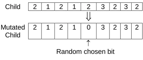
Example of random bit mutation is shown in fig 10. A Random number (0-3) is replaced at the randomly selected place in chromosome.
Child
2
1
2
1
2
3
2 3 2
Mutated
Child
2
1
2
1
0
3
2 3 2
Random chosen bit
Fig 10 : Mutation operation
3.
EXPERIMENT SETUP AND RESULT
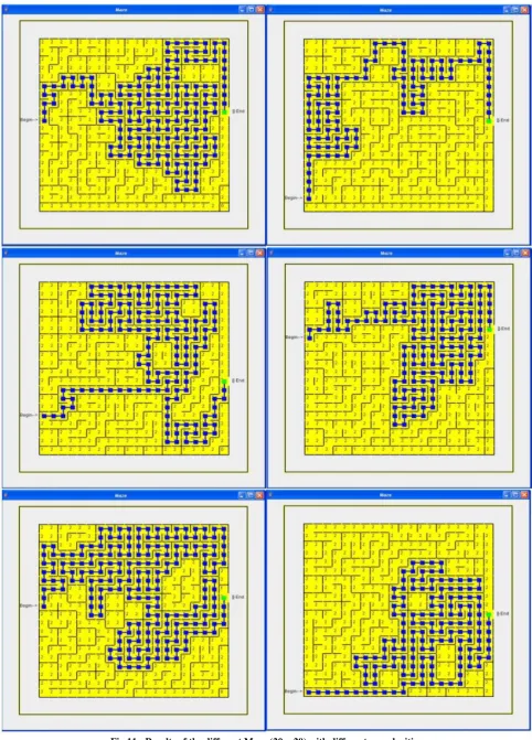
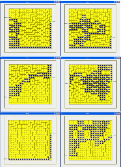
The experiment is conducted JDK 1.6 on Experiment is done with JDK 1.4 on an Intel Core™2 CPU with 2.66 GHZ and 2 GB RAM. The Population size =100, Maximum number of generation = 500, Crossover Rate = 0.8 and mutation rate = 0.1 is used for the purpose of experiment. The length of chromosome is initially considered equal to the length double to the size of the maze (20*2 = 40) for the maze. It is further allowed to gradually increase up to the number of cells available in the maze in the subsequent generations. The optimum solution is found before reaching to the highest value of chromosome length (20 * 20 = 400). The adopted approach is found to give better performance in term of the required number of generation for achieving result. The result obtained for the various 20
20 mazes are shown in the fig
11 and fig 12. It is found that, the population is converged to the best value earlier in case of less complex mazes whereas, whereas it has converged late for the relatively more complex maze structure. The adopted method work on the decision point of choosing the direction change based on the gene value in the chromosome. The other methods such as left wall follower dead end filling, maze solving with imaging work efficiently with the specific mazes only, where as the proposed method uses GA heuristic which leads to the better solution. The adapted method is found to be working successfully on the rectangular mazes considered in theexperiment. There is further scope for adoption of the same method for more complex maze structure having different geometrical structure.
4.
CONCLUSION
The proposed model has been implemented, and the results for the data set used are demonstrated successfully. Modulo operator found to be effective in generating the best results. The mutation operator found to be helpful in generating the new chromosome to avoid the local optima issues. There is further scope for using the methods for more complex maze structure with different geometrical structure than rectangular structure.
5.
ACKNOWLEDGEMENT
Author thanks to the Dr. Tapan Bagchi, Director, SVKM‟s NMIMS, Shirpur campus and Dr. M. V. Deshpande, Associate Dean, MPSTME, Shirpur Campus for providing necessary guidance and infrastructural facilities for conduction of experiment. Author also thanks to Ms. Manisha Kasar, Mr. Nilesh Pawar, and Ms. Shubhangi Patil for their necessary help in data collection.
6.
REFERENCES
[1] Anthony J. Bagnall and Zhanna V. Zatuchna , “On the classification of maze problems” , Foundations of Learning Classifier Systems, Studies in Fuzziness and Soft Computing Volume 183, 2005, pp 305-316.
[2] Oswin Aichholzer, Franz Aurenhammer, David Alberts, and Bernd G¨artner. A novel type of skeleton for polygons. Journal of Universal Computer Science, 1(12):752–761, 1995.
[3] Amazing Mazes, http://fds.oup.Com/ www.oup.co.uk /pdf /0-19-850770-4.pdf
[4] DARWIN C., 1859, The origin of species by means of natural selection, 1859.
[5] Holland John H., 1992. Adaption in Natural and Artificial Systems- Introductory analysis with Application to biology, control and Artificial Intelligence, , Bradford Book edition, The MIT Press, England.,1992.
[6] Goldberg D., 1989. Genetic Algorithm in Search, Optimization, and Machine Learning. Addison Wesley, 1989.
[7] Jianping Cai, Xuting Wan, Meimei Huo, Jianzhong Wu. An Algorithm of Micro Mouse Maze solving. 10th IEEE International Conference on Computer and Information Technology (CIT 2010), 2010
[8] Choubey N.S. & Sonawane S. R., “Comparative Study of various maze solving algorithms”, International Conference in Recent Trends, (i-CORT2012) , IOK-COE, Pune, 2012.
[9] Steve Harrington, “Computer Graphics- A programming Approach”, McGraw-Hill, 1987.
[image:5.595.53.286.297.394.2]