Optimal System Design under Multi Objective Decision making using De Novo Concept: A New Approach

Optimal System Design under Multi-Objective Decision

making using De-Novo Concept: A New Approach

Sayanta Chakraborty

Research Scholar NIT Agartala

Debasish Bhattacharya

Associate Professor NIT Agartala

ABSTRACT

In the realm of multi-objective optimization problem the decision maker only obtains a compromise solution or trade-off solution. These trade-trade-off solutions are the characteristics of sub-optimal, inefficient system configuration. But, it is preferable in all respect to arrive at a feasible solution which optimizes all the objectives at the same time. If this can be achieved then the system is said to be optimally designed. In modern era, the concept of optimal system design (if needed by extending the existed resources) is more important than to optimize a given system with fixed resources. Using De-Novo programming technique one can design an optimal system. The aim of this paper is to present a new approach of applying De-Novo programming technique for optimal design of a system. The applicability of the method has been illustrated through examples. The comparisons of the solutions obtained by the new approach and that of the existing method have been placed.

General Terms

De-Novo Programming, Optimization.

Keywords

De-Novo Programming, Multi-objective optimization, Optimum-path ratio, Optimal system design.

1.

INTRODUCTION

Traditional linear programming technique is a good way of obtaining optimal allocation of fixed or limited resources. But the modern requirement has shifted from allocation of the fixed resources optimally in a given system to design of an optimal system extending the existed resources. De-Novo programming introduced by Zeleny [7,11] deals with this optimal designing of a system. Initially it was designed for single-criteria decision making, later it has been made applicable for multi-criteria decision making [8,9]. The technique is very much computation friendly and thus has become a popular multi-criteria decision making technique for the optimal designing of a system.

To get an insight of the De-Novo [6] technique let us first consider a multi-objective [3] linear decision-making problem.

………..(1)

where and

be the k-th row of C and are the matrices of

dimensions and respectively,

be the m-dimensional

vectors of resources, be the

n-dimensional vectors of decision variables. Here

is the k-th objective.

Let, , , be the optimum value

of the k-th objective function of the problem (1).Then

, the vector of the corresponding q-objective values, is called the ideal point of the system. Let X be the feasible region of the system (1) and

is said to be the ideal

solution if

. In general such an ideal solution may not be feasible since the objectives may be conflicting in nature too. Thus reaching to the ideal point under the given allocation of resources often becomes impossible. But the aim of the decision maker is to reach to the ideal point so that all the objectives could be optimized at the same time. Through De-Novo programming one can easily reach to the ideal point and correspondingly to the ideal solution by extending the existed resources under a given budgetary provision and thus the optimal design of the system could be accomplished.

Let, B be the total available budget and

be the vector of unit prices of m resources. Using the De-Novo programming concept for

optimizing the system (1) one has to find , satisfying

such that the system

is optimized. Thus the De-Novo Programming Problem [8] can be formulated as

…….……….. (2)

The De-Novo concept of the extension of the feasible solution space is illustrated with the help of the figure-1.

where only two objectives (conflicting in nature)

, be the profit objective and be the quality objective for an optimum production planning problem(say) has been considered. In the graph, X denotes the feasible solution space. It is clear that at the portion of the boundary

namely ABCD, both the objectives have higher values in comparison with the other points of the boundary of X and thus those boundary points lying in ABCD part are considered as non-inferior points of the solution space. To

reach to the optimal design , the existing resources should be extended and thus the budget B should be increased.

Now the system (2) is equivalent to

...………..(3)

where [4].

A meta-optimal problem [5] of (3) can be constructed as follows:

s.t.

……….(4)

Solving (4) yields , and . The

value represents the minimum budget to achieve

through under the allocation among the activities.

Since [5] the optimum-path ratio for

achieving the ideal performance for a given budget level B

is defined as .Thus the optimal system design has

been established as , where

and .

In this paper a new approach for the solution of the De-Novo programming problem (2) has been presented. The method of solution has been illustrated through two examples. The solutions derived have been found to agree closely with the solutions obtained by Zeleny’s method.

To accomplish our aim the paper has been divided into five sections. In section-1, the optimal designing of a system by De-Novo technique has been briefly discussed and the related literatures have been cited; in section-2, the new approach has been introduced; in section-3 the solution procedure of the proposed method has been discussed through

two examples; in section-4, the comparison between the new approach and Zeleny’s approach has been done and finally section-5 contains the concluding remarks.

2. NEW

APPROACH

OF

SOLVING

MULTI-OBJECTIVE

DE-NOVO

PROGRAMMING

PROBLEM

Let us recall the multi-objective De-Novo programming problem already introduced in (2):

………..(5).

Through the solution of (5) the optimal allocation of budget is made in such a way that the corresponding resource vector

would maximize all the objectives

simultaneously. It is known that [4] the system (5) is equivalent to

………..(6).

Let, be the vector of the q-objective

values corresponding to the ideal solution Zeleny[10] used the meta-optimal problem (4) for the optimal design of the system (6). Actually the problem (4) aims at a minimum budget which will help to achieve objective values at least as good as the ideal values. Obviously such budget requirement

would be greater than or equal to the given budget . In the new approach the same problem has been viewed in another perspective. It can be considered as a problem of finding the maximum budget required so that the system

could reach at most to the ideal point . It will be seen that both the approaches are in fact equivalent in the sense that both of them lead to the same solution. Under this consideration let us put forward a new problem as follows:

……….(7).

Before proceeding further it is necessary to show that i.e. the ideal solution of system (1) is indeed the optimal solution of (7). This result has been placed in the form of a theorem.

2.1 Theorem

The single-objective LPP,

max , s.t. attains its optimal

Proof

Let be the budget required to reach to the ideal

point. Now it is clear that is a feasible solution of

,

s.t. .

Let be any other feasible solution of the problem (7).To

prove the theorem it is sufficient to show that .

If possible let, .

Let us denote and , then

. This together with our

supposition yields . But is the maximum budget which is required to be allocated so as to

reach to the ideal point under the constraint . Hence

which contradicts the very assumption

, i.e. . Therefore and

hence is the optimal solution of the problem (7) and the theorem is proved.

2.2 Remark

In the proof of the theorem the unique character of the ideal

point and the ideal solution played the decisive role. The ideal solution is the only point common to all the

constraints . This is why the minimum value of the objective function at the lowest point of the upper envelope formed by the constraints is the same as the objective value at the upper point of the lower envelope and thus the problems (4) and (7) have the same optimum solution .In absence of such a common point of intersection of all the constraints the

two problems namely , s.t.

and , , ; may not have a

common optimal solution, e.g. the L.P.P

yields ; whereas

the other problem obtained from the above L.P.P. by reversing the inequalities in the constraints and taking the objective as a minimizing one gives the solution

.

2.3 Note

It can be seen that the value is also the minimum budget

required to attain at least . To see this let us allocate a

budget , among the activities and be the

corresponding resource vector. The optimal solution of the

system (7) yields = and . Now the

feasible region of system (2) corresponding to is a proper

subset to that of . Let, and be the optimal solutions

of (2) corresponding to and respectively. The point

is characterized by i.e.

= , . Therefore for any other point in

the feasible region corresponding to , will not

be satisfied for all . Thus in particular for the point ,

for at least one k . So one can

never reach to the ideal point by allocating the budget

Therefore the optimal solution of (7) simultaneously maximizes all the objectives and the corresponding budget Vx* is the minimum budget required to reach to the ideal

point .

Thus the optimal design of the multi-objective De-Novo programming problem (5) could be achieved by solving the system (7) instead of taking the meta-optimal problem (4).

Solving system (7) the values of , and

can be obtained. Obviously [5]. Now

to achieve the ideal performance related to a given budget

the optimum-path ratio can be defined as . Since

then . Hence

is a solution satisfying the optimum-path ratio.

Also since then and hence

and similarly . Thus the optimal

system can be designed as , where ,

and .

There are two additional types of budgets (other than

.Considering a single objective (say the k-th

one), the budget level required for producing the optimal

with respect to the objective is which is the first

type. The other is . It is defined by [5],

equal to the number of variables, i.e. . It can be shown

that , for

Shi [5] introduced six types of optimum-path ratios:

, , , ,

,

They lead to six different policy considerations and optimal system designs. Comparative economic interpretations of all optimum-path ratios are dependent on the decision maker’s value complex[9].

Through the following real life example the proposed approach of solution of multi-objective De-Novo programming problem is illustrated.

2.2 Example

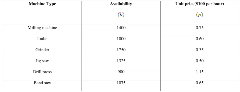
Let us consider a mechanical shop having six machines whose present capacity portfolio is available, measured in machine-hours per week for each machine. Each “hour” of machine capacity has its unit price according to the machine type. The current portfolio of available capacities is furnished through the table-1.

Also the demand of the capacity of the three products has been shown in the table-2.

Here three objectives have been chosen as profit objective, quality objective and worker satisfaction and all the objectives are considered to be equally important. The decision variables

are also supplied, where , respectively denote the number of units of products 1, 2, 3 produced. Thus the multi-objective linear programming problem can be modeled as follows

The initial budget is given as and

the unit prices of the resources are

and .

The above problem was considered by Zeleny[12]. The

problem is to allocate the given budget among the activities to achieve an optimal design of the system. Let

are the optimal resources corresponding to

the given budget The required changes in the resource

components could be effected by purchasing machines of more or of less capacities at their current prices. Then the De-Novo programming model of the problem is as follows:

………(10)

Now it is intended to solve the problem using the proposed approach and for this the given problem is to be re-casted in the form of system (7). This requires the determination of the

ideal point .

The ideal point is determined by considering the objectives one by one together with the given constraints. The three LPPs so obtained are solved and the results are shown.

Thus the ideal point for the considered system is given by

. Now

. Next step is to

rewrite the problem (10) as follows:

s.t.

……….(11)

Solving system (11),one obtains

,

i.e. , -which is

the ideal solution of the system (10) in view of the theorem 2.1. The corresponding budget requirement and resource vector are respectively given by

and

Now ( , , gives the optimal design of the system

under the extended budgetary provision

. But if the system is to be designed under the given budgetary

provision then one has to make use of the

optimum-path ratio introduced by Shi(1995) to find

the corresponding optimal values of maintaining the budget restriction as mentioned. Hence the optimal design of

the product-mix problem i.e. could be obtained by using the optimum-path ratio

and the relations

,

and

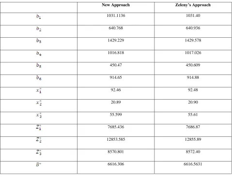
Although by theorem 2.1 the solution obtained by the proposed method and that obtained by Zeleny’s method are same, still for the validation of the proposed method a

comparison of the results obtained by the two methods is shown in table-3.

From the corresponding values obtained by the two approaches it can be seen that the proposed method is an equivalent to that of Zeleny.

To see that the close agreement of the solutions obtained by the two methods in the above example is not a matter of chance, another numerical example has been solved by the two approaches and again an identical result has been derived.

2.3 Numerical Example

……….(12)

The initial budget is given as

and the unit prices of the resources are

, , .

Now the ideal point for the considered system (1) is given by

and .

For determining the optimal design of the system (12) the approach of Zeleny and the proposed one are respectively furnished as system (13) and (14).

s.t.

………(13)

and

………(14)

The solutions of the systems (13) and (14) are found to be exactly same. The identical solution is given by

and and the

corresponding objective values are and

.

This example again validates the correctness of the proposed approach.

3. Conclusion

A remarkable shift from the traditional trade off solution of multi-objective optimization problem to De-Novo optimization towards optimal design of a system could be noticed in problems of economics, portfolio analysis, environmental, unemployment and inflation etc. Thus it is very much pertinent to carry forward the research on De-Novo programming and its solution procedures. In this perspective the present treatise attempts to find out a new approach of solving multi-objective De-Novo programming problem. It is believed that the solution procedure presented here could be implemented in the solution of other derivatives and extension [1,2]of De-Novo programming. The advantage of the proposed approach is that it requires less number of variables (only slack variables) to be introduced in the solution procedure and thus reducing the processing time in comparison with the existing method.

Table 1. Current portfolio of available capacities

Machine Type Availability Unit price($100 per hour)

Milling machine 1400 0.75

Lathe 1000 0.60

Grinder 1750 0.35

Jig saw 1325 0.50

Drill press 900 1.15

Band saw 1075 0.65

Table 2. Demand of the capacity of the products

Machine Type Product 1 Product 2 Product 3

Milling machine 12 17 0

Lathe 3 9 8

Grinder 10 13 15

Jig saw 6 0 16

Drill press 0 12 7

Table 3. Comparison between the results obtained by the two methods

New Approach Zeleny’s Approach

1031.1136 1031.40

640.768 640.936

1429.229 1429.578

1016.818 1017.026

450.47 450.609

914.65 914.88

92.46 92.48

20.89 20.90

55.599 55.61

7685.436 7686.87

12853.585 12855.89

8570.801 8572.40

6616.306 6616.5631

A B

C

Non – inferior Solutions

Feasible Solution X

D

O

Fig 1: De – Novo programming of two objectives

2.

ACKNOWLEDGMENTS

Our thanks to the Department of Mathematics NIT Agartala, for the contribution with resources towards the research.

3.

REFERENCES

[1] Ankan, F., Gungor, Z., 2007, A two-phase approach for multi-objective programming problems with fuzzy coefficients, Information Sciences, (177).

projects planning, International Journal of Production Research, (47) 3503-3523.

[3] Chen, Y.W., 2004, A contractive view on multi-objective programming problems, MCDM, 6-11.

[4] Hesse,M., Zeleny, M., 1987,Optimal system designs: Towards new interpretation of shadow prices in linear programming, Computers and Operations Research,14(4),265-271.

[5] Shi, Y., 1995, Studies on optimum-path ratios in multi-criteria De-Novo programming problems, Computers Math. Applic., 29(5) 43-50.

[6] Zeleny, M., 1990, De-Novo Programming, Ekonomicko-matematicky obzor,(26) 406-413.

[7] Zeleny, M.,1976,Multi-objective design of high-productivity systems, In: Proc. Joint Automatic Control Conf., paper APPL9-4, New York.

[8] Zeleny, M., 1982,Multiple Criteria Decision Making. New York, McGraw-Hill.

[9] Zeleny, M., 1998, Multiple Criteria Decision Making: Eight concepts of optimality, Human Systems Management, 17(2), 97-107.

[10]Zeleny, M., 2009, On the essential multidimensionality of an Economic problem: Towards tradeoffs-free economics, Acta Universitatis Carolinae Oeconomica, (3) 154-175.

[11]Zeleny, M., 1981, On the squandering of resources and profits via linear programming. Interfaces, 11(5), 101-107.