A Comprehensive Active Contour Model

35

A Comprehensive Active Contour Model

Abhinav Chopra

Amity University

Uttar Pradesh, India

Bharat Raju Dandu

Amity University

Uttar Pradesh, India

ABSTRACT

Image segmentation is one of the substantial techniques in the field of image processing. It is excessively used in the field of medicine provides visual means for identification, inspection and tracking of diseases for surgical planning and simulation. Active contours or snakes are used extensively for image segmentation and processing applications, particularly to locate object boundaries. Active contours are regarded as promising and vigorously researched model-based approach to computer assisted medical image analysis. However, its utility is limited due to poor convergence of concavities and small capture range. Many subsequent models have been introduced in order to overcome these problems. This paper reviews the traditional model, the Gradient vector flow (GVF) model and the balloon model for different images and proposes a model which can provide the most accurate segmentation.

Keywords:

Active contour models, edge detection, gradient vector flow, balloon model, image segmentation, snakes.

1.INTRODUCTION

Segmentation is the process of splitting the image into several parts like objects (also called foreground or background. Active contours [1] or snakes provide an effective way of segmentation [2] of curves defined within the image domain that can move under the influence of external and internal forces. These forces are defined such that the snake will shrink wrap to an object boundary. This method is widely used in many applications, including motion tracking, edge detection and segmentation.

There are two types of active contour models in literature today: - parametric active contours and geometric active contours [3][4]. Our main focus here is on parametric contours. Parametric active contours synthesize parametric curves within an image domain and allow them to move towards desired features, usually edges. Typically the curves are drawn towards the edges by potential forces, which are defined to be the negative gradient of a potential function. Additional forces like the potential forces[5] and pressure forces together comprise the external forces. There are also internal forces designed to hold the curve together (elastic forces) and to keep it from bending too much (bending forces).

There are two main difficulties we face during the parametric active contour algorithm. First, the active contours have difficulties progressing into boundary concavities[6][7]. The second problem is that the initial contour must in general, be close to the true boundary or else it will predict an incorrect

result. Most of the methods that are proposed to solve the above problems are ineffective in solving both issues and end up creating more difficulties.

In this paper we represent distinct active contour models to help resolve the problems mentioned above. Firstly, the

traditional model and its shortcomings. Then the balloon model or the expanding snake model helps resolve the problem of small capture range. When the approximate boundary of an object is unknown the traditional model fails to provide accurate results, in such situations using the balloon model shows robustness. Finally, the gradient vector flow (GVF) model[8] which forces active contours into concave regions. GVF is computed as a diffusion of the gradient vectors of a gray-level or binary edge map derived from the image. We discuss the above models by using different types of images i.e. regular without concavities and irregular images with concavities.

The major advantage of using these models over the traditional model is that it can be initialized far from the boundary since it has a large capture range. And unlike pressure forces, it does not require prior knowledge about when to shrink or expand towards the boundary.

2.MATERIAL AND METHODS

2.1.Parametric Snake Model

The contour [1] is defined in the (x, y) plane of an image as a parametric curve

v

(

s

) = (

x

(

s

),

y

(

s

))

Contour is said to possess energy (

E

snake) which is defined as

the sum of the three energy terms.

The energy terms are defined cleverly in a way such that the final position of the contour will have a minimum energy (Emin)

Therefore our problem of detecting objects reduces to an energy minimization problem.

Internal Energy (Eint) depends on the intrinsic properties of

the curve and is the sum of elastic energy and bending energy.

36 Weight (s) allows us to control elastic energy along different

parts of the contour.

Considered to be constant for many applications

.

Bending Energy (

Ebending

): The snake is also considered to behave like a thin metal strip giving rise to bending energy. It is defined as sum of squared curvature of the contour.

(s) plays a similar role to (s). Bending energy is minimum for a circle.

Total internal energy of the snake can be defined as:-

External energy (

Eext

) of the contour is derived from the image so that it takes on its smaller values at the function of interest such as boundaries[10]. Define a function Eimage

(x,y

)

so that it takes on its smaller values at the features of interest, such as boundaries.

Key rests on defining

E

image

(x,y).

Some examples

A.

B.

Energy and force equations:The problemcurrently on hand is to find a contour v(s) that minimize the energy functional

Using variational calculus and by applying Euler-Lagrange differential equation we get following equation

Equation can be interpreted as a force balance equation.

F

int

+ F

image

= 0

Each term corresponds to a force produced by the respective energy terms. The internal force Fint discourages stretching and bending while the external potential force Fimage pulls the snake toward the desired image edges

.

Solving the Euler equation:-

Consider the snake to also be a function of time i.e

.

If RHS=0 we have reached the solution. On every iteration update control point only

if new position has a lower external energy. Snakes are very sensitive to a false local minimum which leads to wrong convergence.

2.2

Weakness of Traditional Snakes

An example of behavior of traditional snake is shown in fig. 3(b) and fig. 4(b). In fig. 4(b) we can see that it has boundary concavity on the side are left vacant. This snake formulation is a result of Euler’s equation and we can see that it remains split across the concave region.

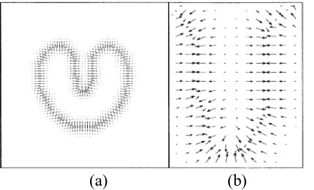
The reason for the poor convergence of this snake as seen in fig. 1(b) is because the forces point horizontally in opposite direction.

37

(a)

(b) (a) (b)

Fig. 1 (a) traditional potential forces and (b) close- up Fig. 2 (a) traditional distance forces and (b) close-up

2.3.Balloon Model

The snake model originally introduced by Kass has been further developed by modified in recent years. The balloon model or the expanding snake mode[9] is one of the examples of this. Unlike, the traditional snake that shrinks wraps to the image boundary, this snake model expands outwards.

This model is based on an additional inflation force applied to give stable results. A snake which is not close to contours is not attracted by them. The curve behaves like a

balloon which is inflated. When it passes by edges, will not be trapped by spurious edges and only is stopped when the edge is strong. The initial guess of the curve not necessarily is close to the desired solution. Pressure force is added to the internal and external forces[11].

The expansive behavior is achieved by modifying the

values of f

x

; f

y

as followed

where n(s) is the unit principal normal vector to the curve at point v(s), and k1 is the amplitude of this force. k1 and k are chosen such that they are of the same order, which is

smaller than a pixel size and k is slightly larger than k1 so an edge point can stop the Inflation force. The curve then expands and it is attracted and stopped by edges as before. The smoothing effect with the help of the inflation force then removes the discontinuity and the curve then passes through the edge.

2.4.Gradient Vector Flow Snake

The overall approach is to use the force balance condition as a starting point to design the snake. This parametric curve thus formed is called GVF snake[12]

.

Gradient Vector Flow:-The GVF field is defined to be a vector field[13][14]

Force equation of GVF snake is,

V(x,y

) is defined such that it minimizes the energy functional,

(a)

(b)

[image:3.595.50.275.86.222.2] [image:3.595.303.523.86.220.2]

38

(a)

(b)

(c)

Fig.4 (a) snake boundary, (b) snake not able to move into concavities in the traditional or balloon model and (c) complete convergence of the boundary in GVF model

f(x,y) is the edge map of the image.

GVF field can be obtained by solving following equations

2

Is the Laplacian operator.

The above equations are solved iteratively using time derivative of u and v. These equations provide further intuition behind the GVF formulation[15]. We note that in the homogenous region the second term in both regions is zero because the gradient of f(x, y) is zero.

3.

RESULTS

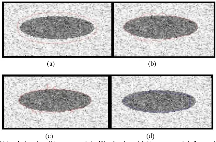
When tested on an image with regular shape (rectangle), with no concavities (fig.3) and with no noise present in the image, all the three models were able to form a complete boundary, but the GVF snake(fig.3(b)) showed the highest rate of convergence. Tests on an image (scissors) with concavities (fig.4), showed what we had expected from the theoretical studies. Neither original nor balloon snake managed to enter the concavity (fig.4 (b)). The GVF snake (fig.4 (c)) did so in very few iteration. When tested on an image which was corrupted by noise, traditional (fig.5 (b)) and especially balloon snake (fig.5(c)) were distracted but still able to extract the boundary appropriately. The GVF snake (fig.5 (d)), on the other hand, became unstable and “broke” the boundary

(a)

(b)

(c)

(d)

[image:4.595.95.494.86.223.2] [image:4.595.117.489.492.736.2]

39

4. CONCLUSION

We have successfully reviewed the three distinct snake models i.e. traditional snake model, balloon snake model and the GVF snake model by applying them to different images and studied their result. Different models provide varied accuracy based on the type of images. As we saw in figure 4 how the GVF model was successful in forming boundaries by entering concavities, while the other two models were not able to enter these areas. Similarly we encounter wide-ranging types of images for segmentation, specially in medicine where cancer cells vary in structure depending upon their location. Hence we can conclude that a combination of these models would provide a robust and comprehensive method for segmentation for various types of images.

5. REFERENCES

[1] M. Kass, A. Witkin, and D. Terzopoulos, “Snakes: Active contour models,” Int. J. Comput. Vis., vol. 1, pp. 321-331, 1987.

[2] H. Tek and B. B. Kimia, “Image segmentation by reaction-diffusion bubbles,” in Proc. 5th Int. Conf. Computer Vision, 1995, pp. 156-162.

[3] V. Caselles, F. Catte, T. Coll, and F. Dibos, “A geometric model for active contours,” Numer. Math., vol. 66, pp. 1-31, 1993.

[4] R. Malladi, J. A. Sethian, and B. C. Vemuri, “Shape modeling with front propagation: A level set approach,”IEEE Trans. Pattern Anal. Machine Intell., vol. 17, pp. 158-175, 1995.

Englewood Cliffs, NJ: Prentice-Hall, 1989

[6] C. Davatzikos and J. L. Prince, “Convexity analysis of active contour models,” in Proc. Conf. Information Science and Systems, 1994, pp.581-587.

[7] H. Tek and B. B. Kimia, “Image segmentation by reaction-diffusion bubbles,” in Proc. 5th Int. Conf. Computer Vision, 1995, pp. 156-162.

[8] C. Xu and J. L. Prince, “Gradient vector flow: A new external force for snakes,”

[9] L. D. Cohen and I. Cohen, “Finite-element methods for active contour models and balloons for 2-D and 3-D images,” IEEE Trans. Pattern Anal. Machine Intell., vol. 15, pp. 1131-1147, Nov. 1993.

[10] L. D. Cohen. On active contour models and balloons.CVGIP: Image Understanding, 53(2):211–218, Mar. 1991

[11] R. Courant and D. Hilbert, Methods of Mathematical Physics, vol 6.

[12] B. K. P. Horn and B. G. Schunck, “Determining optical flow,” Artif.Intell., vol. 17, pp. 185–203, 1981.

[13] C. Xu and J. L. Prince. Snakes, shapes, and gradient vector flow. IEEE Trans. on Image Processing. to appear.

[14] C. Xu and J. L. Prince. Snakes, shapes, and gradient vector flow. Technical Report JHU-ECE TR96-15, The Johns Hopkins University, Oct. 1996.