88
APPLICATION OF SUPPORT VECTOR REGRESSION FOR
JAKARTA STOCK COMPOSITE INDEX PREDICTION WITH
FEATURE SELECTION USING LAPLACIAN SCORE
1ZUHERMAN RUSTAM, 2KHADIJAH TAKBIRADZANI
1Senior Lecturer, Department of Mathematics, Faculty of Mathematics and Natural Science, University of
Indonesia, DEPOK, INDONESIA
2Undergraduate Student, Department of Mathematics, Faculty of Mathematics and Natural Science,
University of Indonesia, DEPOK, INDONESIA E-mail: 1[email protected], 2[email protected]
ABSTRACT
Researchers and investors have been searching for accurate model to predict the stock value. An accurate model prediction could gain profits for investors. According to Indonesia Stock Exchange, stock is becoming one of the most popular financial instrument in Indonesia. Investors take the smaller sample called index that represent the whole because it would be too complicated to record every single security that trades in the country. There are many stock indices in the world, one of them, is Jakarta Composite Index (JKSE). One of the benefits of following the stock indices value is to reduce the loss in investment. Thus, this paper is focused in supervised learning method to solve regression problem, Support Vector Machines for Regression (SVR). There are fourteen technical indicators calculated in this paper. Laplacian score will be calculated for each fourteen technical indicators. Laplacian score is calculated to mirror the locality preserving power. Support Vector Machines for Regression (SVR) with feature selection using Laplacian Score is the proposed methodology with Jakarta Compostie Index (JKSE) are considered as input data. The best model is the prediction model with thirteen features and 30% training data which has value of Normalized Mean Squared Error (NMSE) is 1.30691E-07
Keywords: Laplacian Score; Support Vector Machines for Regression (SVR); Jakarta Composite Index (JKSE); Stock
Price Trend Prediction.
1. INTRODUCTION
One option to achieve the needs of life in the future is through investment. There are many ways to invest our fund, in terms of investment tools, one of them is stock. One of the type of security that signifies ownership and is a claim for a portion of a company’s assets and revenues is stock. Since stock is promising in high profit return, the goal of stock trading is to gain high profits. Not only stock trading is promising in high return profit, but stock also having high potential for high loss. The reason is because stock market is an unstable, complex, evolutionary, nonlinear and complex system of dynamic change [1-3]. Stock market is contrived by many causes such as significant economic approaches, government commandment, the change of political situation, investor’s state of mind, the future economy, and so on [4].
Predicting stock indices could improve investor’s market exchange strategies. There are many ways to predict indices stock value movement, one of them is through technical analysis which use specific indicators. Technical indicators are the key tools for look after the movement of stock price and helping investors to make trading decisions [5,6]. However, those specific indicators do not perform very well in predicting stock market indices accurate [4]. With the help of technical indicators, there are many prediction methods realize in the research articles which predict the stock indices movement. A total of fourteen technical indicators are used in this paper.
89 can be used as inputs, but the irrelevant and correlated data could degrade the performance of SVR. To overcome this problem, all technical indicators will be selected. Laplacian Score will be used as feature selection. Laplacian Score could be used both in supervised or unsupervised way. Laplacian Score will be calculated to reflect the feature’s locality preserving power [8]. This paper focused to predict stock indices movement in Jakarta Composite Index (JKSE) using Support Vector Machines for Regression (SVR) with feature selection using Laplacian Score.
2. LITERATURE REVIEW
In this section, we will discuss Related Works in this paper, Stock Composite Index, Technical Analysis, Laplacian Score, and Support Vector Machines for Regression (SVR).
2.1 Related Work
There are many related researches in recent years. Support Vector Machines (SVM) have been used well to predict stock price index and stock price movements. Neural networks widely used to modelling financial time series and it successfully worked [9]. In 2014, G. Lin, H. Guo, and J. Hu implemented Support Vector Machines (SVM) filter based on correlation to select a good subset of financial indexes [10]. Support Vector Machine (SVM) stock selection model within Principal Component Analysis (PCA) is proposed by H. Yu, C. Rongda, and G. Zhang in 2014, is applied to A-share index of Shanghai Stock Exchange, contributes the periodical earnings of stock portfolio to surpass the A-share index of Shanghai Stock Exchange [11].
2.2 Stock Composite Index
Stock composite index is one of the stock market price indexes, that measures the changes over time in the stock price (or other financial assets) traded in particular stock markets. These indexes are calculated daily, or a couple times a day in the business hours. By knowing the the value of the stock composite index, it concludes the trend of stock price movements on the market, whether increase, down, or stable. If the Stock Composite Index in downtrend, then it’s not a right time to invest because the stock market is not in a profitable condition. The trend of stock price movements information can be used by Investors to make decision to hold, buy, or sell a stock or some stocks.
2.2.1 Technical Analysis
Technical analysis is a way to
evaluate investments. Technical analysis is also a way to identify trading opportunities by analyzing statistical trends obtained from trading history and trading activity, such as close price, high price, low price and volume. It is different from fundamental analysis. Fundamental analysis is a method to evaluate a company’s essential value, meanwhile technical analysis focus on the shape of price movements, signals of trading and various other analytical charting tools to evaluate a company’s advantages and flaw.
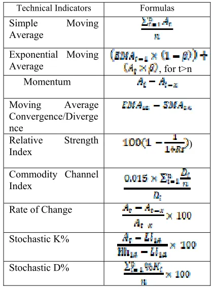
[image:2.612.320.529.404.689.2]Technical indicators is needed before we use technical analysis. Technical indicators are mathematical formulation which use historical price data such as low price, high price, close price, and volume. Below in Table 1 is technical indicators that used in this paper based on the previous study [12-14]:
Table 1: Technical Indicators used in this paper
Technical Indicators Formulas
Simple Moving Average
Exponential Moving
Average , for t>n Momentum
Moving Average Convergence/Diverge nce
Relative Strength
Index )
Commodity Channel Index
Rate of Change
Stochastic K%
90 In Table 1, the adjusted close price of day t is , n explained number of trading days used, is Exponential Moving Average value yesterday (t-1), is the smoothing coefficient or weight coefficient, where Rs is
, the is the gain from the change in adjusted close price (increasing price change) and is loss from the change in adjusted close price (decreasing price change), represents the difference between typical price and the average of typical price in some period where typical price is High Price plus Low Price plus Adjusted Close Price, and are the lowest price and the highest price for the last 14 days.
2.3 Laplacian Score
Feature selection can be categorized as “wrapper” and “filter” method [15]. The “wrapper” method as feature evaluation using the learning algorithm that will be used yet. Hence, the selection process is “wrapped” over the learning algorithm. The intrinsic properties of the data are being checked by algorithms based on the filter model to evaluate features before the learning task. In 2005, X.F. He, D. Cai, and P. Niyogi proposed algorithm called Laplacian Score. Laplacian Score is a novel feature selection algorithm. Thus, the algorithm is as follows according [8]:
1.) Build a closest neighbor graph G with m nodes. For each observation, put an edge between nodes i and g for that observation if xi and xj are “close”, i.e. if
another observation is one of its k-nearest neighbor's (xi is between k-nearest
neighbors of xj, and vice versa). For
supervised algorithm, define an edge if they share the same label.
2.) If any two nodes from observations are linked (for example: nodes i and j), define the weight matrix:
(1) Where t is suitable constant and for otherwise.
3.) For each feature, define:
r = , D = diag(S1),
1= , . Let:
(2)
4.) For each feature, calculate the Laplacian Score as follows:
(3)
The good feature is a feature with the bigger Sij,
hence the Laplacian Score likely to be small.
2.4 Support Vector Machines for Regression
(SVR)
Support Vector Machines for regression (SVR) is a supervised Machines learning technique to solve nonlinear regression problem. Vapnik firstly introduced Support Vector Machines in 1995. In Support Vector Machines for
Classification, we use linear learning method and the kernel trick to search the main characteristics of maximum margin method [16]. For regression problems, we need to improve an estimator because the traditional least-squares estimator may not be decent in front of outliers. This robust estimator is called -insensitive loss function. ε-Insensitive Loss Function according to [17]:
Let f be a actual value of X. The ε-insensitive loss function Lε(x, y, f ) is defined as:
Lε(x, y, f ) = |y − f (x)|ε=max(0, |y − f (x)| − ε) (4)
With the establishment of ε-insensitive loss function, Support Vector Machines (SVM) have been extended to unravel non-linear regression problems and it showed an exquisite work in financial time series forecasting [15]. Different with Support Vector for Classification (SVC), Support Vector Regression (SVR) has an supplementary free parameter ε. The two free parameters which are εand C command the Vector Classification dimension of the resemble function as in [16]:
91 when we change the bias v = 0. The model prediction we will be used is [16]:
(6) where and is the Lagrange multiplier,
is the kernel function, is the input vector, and v is a bias.
3. THE PROPOSED METHOD
This paper proposed the application of Support Vector Regression (SVR) with feature selection using Laplacian Score. Laplacian Score is used in preprocessing data. Using Laplacian Score, the prediction model will become more effective because Laplacian Score helps us to choose a good feature. Laplacian Score is calculated to mirror the feature’s locality preserving power [8]. The fundamental idea of Laplacian Score is if the two data points are connected if they are near each other. Adjusted close price historical data is collected from yahoo finance. We treated adjusted close price as raw input data to transform to be technical indicators’ values because technical indicators is used as input variables. However, the stock data samples have different values and scales. Thus, the data must be normalized to make the prediction model effective.
3.1 Data Sets
The authors used one of Stock Composite Index in Indonesia, which is Jakarta Composite Index (JKSE). This index represent of all stocks that traded on Indonesia Stock Exchange (IDX). Authors prefer used adjusted close price to close
price. Based on Investopedia, adjusted close price
is a close price which has been adjusted with company’s corporation action (e.g. stock split) on the day. Thus, adjusted close price is more represent the whole than close price. We taken 491 data points from yahoo finance. The corresponding time period is from 24th October 2014 to 26th
October 2016. Moving Average (MA), Moving Average, Stochastic Oscillator (SO), Rate of Change (ROC), Momentum (MOM), and Convergence Divergence (MACD) are fourteen technical indicators as input data.
3.2 Data Preprocessing
The step of authors’ data preprocessing is technical analysis, normalization data, and
Laplacian Score. Technical analysis use technical indicators which are obtained from historical with mathematical formulation [20]. The historical data that used for technical indicators are adjusted close price, low price, and high price. The technical indicators formula that used in this study is the formula according to [12-14].
As previously explained, we need to normalize the data to adjust the content of all feature. We use the formula below to normalize the data into intervals [-1,1] according to [21]:
(7)
where x(t) is technical indicator A on the t-th day, x’(t) is the new normalized technical indicator A on the t-th day, max A is the maximum number of technical indicator A, min A is the minimum number of technical indicator A. Max’A is the new normalized maximum number of technical indicator A, which is 1. Min’A is the new normalized minimum number of technical indicator A, which is -1.
After successfully finished normalize the data, Laplacian Score will be used to find the good features.
3.3 Feature Selection
Variance data may find the features that valuable for symbolize the data. However, there is no argument for assuming that the features need to be symbolize for fussy among data in particular classes. The base of Laplacian Score is if two data points are near each other, then the two data points are probably connected to the same topic. In the previous study of He, Cai, and Niyogi have researched of Laplacian Score for face pattern recognition and clustering [8]. It showed that Laplacian Score performs better than variance for feature selection. Authors inspired by their output to try it in predicting stock model.
92 fourteen feature, we run Support Vector Regression (SVR) program from one feature, two feature, and so on until fourteen features. We use from 10% data for train, 20% data for train, until 90% data for train to find the best model.
3.4 Performance Criteria
There are a lot of formula to evaluate the performance of the prediction model. The commonly used formulas are Normalized Mean Squared Error (NMSE), Root Mean Squared Error (RMSE), and Mean Absolute Percentage Error (MAPE). In this study, the authors pick Normalized Mean Squared Error (NMSE) to evaluate the performance.
Normalized Mean Squared Error (NMSE) is the sizes of the deviation between the observed and predicted values. The smaller values of Normalized Mean Squared Error (NMSE) showed that the nearer are the predicted values to observed values. The formula of Normalized Mean Squared Error (NMSE) test set based on [22] is:
(8)
(9)
Where represent the observed value, is the predicted value, represent the mean of observed output values.
4. EXPERIMENTAL RESULT
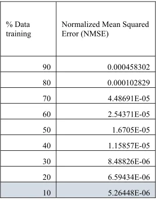
[image:5.612.313.467.119.316.2]The model prediction using Support Vector Regression (SVR) using feature selection which have from one feature only, two features only, three features only, and so on have Normalized Mean Squared Error (NMSE) showed in table below:
Table 2: Table with one feature Normalized Mean
Squared Error (NMSE)
% Data
training Normalized Mean Squared Error (NMSE)
90 0.000458302
80 0.000102829
70 4.48691E-05
60 2.54371E-05
50 1.6705E-05
40 1.15857E-05
30 8.48826E-06
20 6.59434E-06
[image:5.612.309.470.373.572.2]10 5.26448E-06
Table 3: Table with two features Normalized Mean Squared Error (NMSE)
% Data
training Normalized Mean Squared Error (NMSE)
90 0.000458618
80 0.000102391
70 4.38458E-05
60 2.50207E-05
50 1.64048E-05
40 1.16126E-05
30 8.40683E-06
20 6.58523E-06
93
Table 4: Table with three features Normalized Mean Squared Error (NMSE)
% Data training
Normalized Mean Squared Error (NMSE)
90 3.01059E-05
80 7.27805E-06
70 4.10639E-06
60 3.50553E-06
50 3.34952E-06
40 3.37603E-06
30 3.59141E-06
20 3.91128E-06
10 4.04359E-06
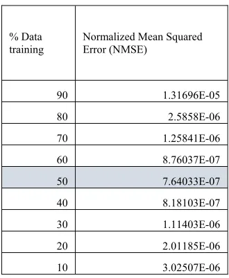
Table 5: Table with four features Normalized Mean Squared Error (NMSE)
% Data
training Normalized Mean Squared Error (NMSE)
90 1.31696E-05
80 2.5858E-06
70 1.25841E-06
60 8.76037E-07
50 7.64033E-07
40 8.18103E-07
30 1.11403E-06
20 2.01185E-06
[image:6.612.89.244.134.333.2]10 3.02507E-06
Table 6: Table with five features Normalized Mean Squared Error (NMSE)
% Data training
Normalized Mean Squared Error (NMSE)
90 1.24997E-05
80 2.26653E-06
70 1.01299E-06
60 6.57682E-07
50 5.18138E-07
40 4.70613E-07
30 4.53615E-07
20 9.37157E-07
10 2.16486E-06
Table 7: Table with six features Normalized Mean Squared Error (NMSE)
% Data training
Normalized Mean Squared Error (NMSE)
90 1.05128E-05
80 1.91418E-06
70 8.98161E-07
60 5.59771E-07
50 4.28761E-07
40 3.94075E-07
30 4.19077E-07
20 8.27126E-07
[image:6.612.89.254.372.572.2] [image:6.612.312.477.385.586.2]94
Table 8: Table with seven features Normalized Mean Squared Error (NMSE)
% Data
training Normalized Mean Squared Error (NMSE)
90 1.12015E-05
80 1.96719E-06
70 9.65403E-07
60 5.95523E-07
50 4.62723E-07
40 3.99315E-07
30 4.08637E-07
20 7.84993E-07
[image:7.612.89.245.118.317.2]10 1.99565E-06
Table 9: Table with eight features Normalized Mean Squared Error (NMSE)
% Data training
Normalized Mean Squared Error (NMSE)
90 9.89232E-06
80 1.7603E-06
70 7.90752E-07
60 4.34794E-07
50 3.15894E-07
40 2.9138E-07
30 2.58036E-07
20 4.10765E-07
[image:7.612.312.468.356.552.2]10 1.36712E-06
Table 10: Table with nine features Normalized Mean Squared Error (NMSE)
% Data
training Normalized Mean Squared Error (NMSE)
90 9.13715E-06
80 1.5969E-06
70 7.04076E-07
60 3.8784E-07
50 2.55403E-07
40 2.27592E-07
30 2.13344E-07
20 2.93855E-07
10 9.23255E-07
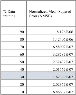
Table 11: Table with ten features Normalized Mean Squared Error (NMSE)
% Data training
Normalized Mean Squared Error (NMSE)
90 8.176E-06
80 1.42406E-06
70 6.58002E-07
60 3.28787E-07
50 2.32432E-07
40 2.01562E-07
30 1.62379E-07
20 2.02352E-07
[image:7.612.89.244.356.553.2]95
Table 12: Table with eleven features Normalized Mean Squared Error (NMSE)
% Data training
Normalized Mean Squared Error (NMSE)
90 7.41191E-06
80 1.42647E-06
70 6.18118E-07
60 3.12599E-07
50 2.17836E-07
40 2.01365E-07
30 1.601E-07
20 1.97922E-07
10 5.55335E-07
Table 13: Table with twelve features Normalized Mean Squared Error (NMSE)
% Data training
Normalized Mean Squared Error (NMSE)
90 4.71417E-06
80 9.8309E-07
70 4.92472E-07
60 2.54548E-07
50 1.72879E-07
40 1.5441E-07
30 1.44631E-07
20 1.55957E-07
[image:8.612.89.244.134.333.2]10 4.82723E-07
Table 14: Table with thirteen features Normalized Mean Squared Error (NMSE)
% Data training
Normalized Mean Squared Error (NMSE)
90 4.56975E-06
80 8.68687E-07
70 5.00036E-07
60 2.72656E-07
50 1.89223E-07
40 1.46228E-07
30 1.30691E-07
20 1.50639E-07
10 4.72108E-07
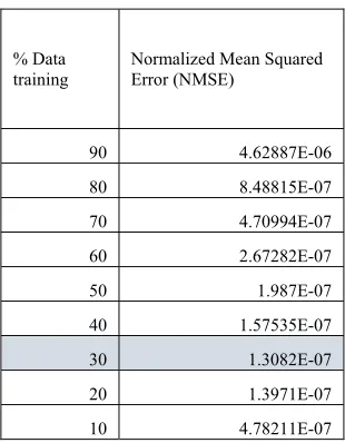
Table 15: Table with fourteen (ALL) features Normalized Mean Squared Error (NMSE)
% Data training
Normalized Mean Squared Error (NMSE)
90 4.62887E-06
80 8.48815E-07
70 4.70994E-07
60 2.67282E-07
50 1.987E-07
40 1.57535E-07
30 1.3082E-07
20 1.3971E-07
10 4.78211E-07
[image:8.612.313.468.386.585.2] [image:8.612.89.244.387.586.2]96 gives the same NMSE value, then we better use 30% training data, since it will shorten the running time of the program.
From all of the tables, as you can see the smallest NMSE is obtained by using thirteen features with 30% data training.
5. CONCLUSION AND FUTURE WORKS
The application of Support Vector Regression (SVR) with feature selection using Laplacian Score to forecast the price index movement offered a good result since it has relatively small NMSE values, which below 0.1. Even though the value of NMSE has different output for each %data training and features. For example, in Table 14, using only thirteen features, the best output is with only 30% data training, but for only one feature the best model is with 90% data training. Some of the data obtain the smallest NMSE value both with and without feature selection, it may be better to use less feature for time eficiency.
Moreover, the model and output influenced by the types of data, the types of feature, and %data training used. Therefore, an accurate stock price prediction model is needed so investors could gain profits and minimize risks. For other work in the future, we will use other technical indicators or use historical data only for input variables and use other data than Jakarta Composite Index, or using other data such as medical data, other financial data, and so on.
6. ACKNOWLEDGEMENTS
This research was supported financially by the Indonesia ministry of Research and Higher of Education, with PDUPT 2018 research grant scheme ID number 389/UN2.R3.1/HKP05.00/2018.
REFERENCES
[1] Ince, Huseyin. (2007). Kernel principal component analysis and support vector machines for stock price prediction. Iie Transactions. 39. 10.1080/07408170600897486.
[2] Hall, J.W. (1994) “Adaptive selection of US stocks with neural nets.” G.J. Deboeck (Ed.), Trading On the Edge: Neural, Genetic, and Fuzzy Systems for Chaotic Financial Markets, Wiley, New York: 45–65.
[3] Guegan, D. (2009). Chaos in economics and finance. Annual Reviews in Control, 33 , 89– 93.
[4] Y. Chen and Y. Hao, A feature weighted support vector Machines and K-nearest neighbor algorithm for stock market indices prediction, Expert Systems With Applications 80 (2017) 340–355.
[5] R. Dash and P. K. Dash, A Hybrid Stock Trading Framework Integrating Technical Analysis with Machine Learning Techniques, The Journal of Finance and Data Science 2 (2016) 42–57
[6] Kirkpatrick, Charles D., Dahlquist, Julie R.
(2006). Technical Analysis: The Complete
Resource for Financial Market Technicians. Financial Times Press. ISBN 0-13-153113-1.
[7] C. Cortez and V. Vapnik, Support Vector Networks, Machines Learning, 20 273–297, 1995.
[8] X.F. He, D. Cai, and P. Niyogi. (2005). Laplacian score for feature selection, in: Advances in Neural Information Processing Systems. Cambridge.
[9] T. Kimoto, K. Asakawa, M. Yoda, and Takeoka (1996), “Stock market prediction system with modular neural networks.” R.R. Trippi, E. Turban (Eds.), Neural Networks Finance Investing: Using Artificial Intelligence to Improve Real-World Performance, Irwin Publ., Chicago: 497–510.
[10]Y. Lin., H. Guo.,and J. Hu (2013). An svm-based approachf orstock market trend prediction in: In Neural Networks (IJCNN), The 2013 International Joint
Conference.IEEE:1–7
[11]H. Yu., R. Chen., and G. Zhang (2014). A svm stock selection model within pca. Procedia computer science. 31:406–412.
97 Trend Deterministic Data Preparation and Machine Learning Techniques, Expert Syst. Appl. 42 (2015) 259–268.
[13]Y. Kara, M. A. Boyacioglu, and Ö. K. Baykan, Predicting Direction of Stock Price Index Movement using Artificial Neural Networks and Support Vector Machines: The Sample of Istanbul Stock Exchange, Expert Syst. Appl. 38 (2011) 5311–5319.
[14]B. M. Henrique, V. A. Sobreiro, and H. Kimura, Stock price prediction using support vector regression on daily and up to the minute
prices, The Journal of Finance and Data
Science Volume 4, Issue 3, September 2018, Pages 183-201.
[15]R. Kohavi and G. John, “Wrappers for Feature Subset Selection,” Artificial Intelligence, 97(1-2):273-324, 1997.
[16] X. Wu, and V. Kumar, “The Top Ten Algorithms in Data Mining”, Taylor & Francis Group, LLC, pp. 50-51, 2009.
[17] N. Cristianini and J. Shawe-Taylor. An Introduction to Support Vector Machines and
OtherKernel-based Learning Methods,
Cambridge University Press, 2000.
[18]S. Mukherjee, E. Osuna, F. Girosi, Nonlinear prediction of chaotic time series using support vector machines, in: NNSP’97: Neural Networks for Signal Processing VII: Proceedings of the IEEE Signal Processing Society Workshop, 1997, Amelia Island, FL, USA, pp. 511–520.
[19]C. M. Bishop, “Pattern Recognition and Machine Learning”, Springer, New York, 2006.
[20] Z. Rustam, D. F. Vibranti, and D. Widya, “Predicting The Direction of Indonesian Stock Price Movement using Support Vector Machines and Fuzzy Kernel C-Means”, 3rd International Symposium on Current Progress in Mathematics and Sciences, Bali, 2017 [21]M. Kumar, Thenmozhi. M, “Forecasting Stock
Index Movement: A Comparison of Support Vector Machines and Random Forest”, Indian Institute of Capital Markets 9th Capital Markets Conference Paper, 2006.