A Simulations and Data Fit Mathematical Modeling of G CSF Drug Treatment

Journal of Chemical and Pharmaceutical Research, 2016, 8(6):223-232

Research Article

_{CODEN(USA) : JCPRC5}

ISSN : 0975-7384

A Simulations and Data Fit Mathematical Modeling of G-CSF Drug

Treatment

S. Balamuralitharan

Faculty of Science and Humanities, Department of Mathematics, SRM University, Kattankulathur-603 203, Tamil Nadu, India

_____________________________________________________________________________________________

ABSTRACT

The purpose of this paper is to study the G-CSF (Granulocyte-Colony Stimulating Factor) treatment of a simulations and data fit mathematical modeling of CN (Cyclical Neutropenia) with neutrophil count. This model is useful to account for the features of untreated G-CSF. It is also useful for treatment of dogs with CN. Therefore this model is considered as an accomplished one. There is fitting parameters for 3 days and not for 4 dogs for estimation or evaluation. It is also essential and necessary to model the more samples for increase in Neutrophil amplification. The proposed interventions are practical. It may reduce the amount of G-CSF. It required potential maintenance. Sometimes, it may even improve the treatment effects too. This model gives us good result in treatment. The changes would be practical and reduce the risk side as well as the cost of treatment in G-CSF. By using a four GC’s (grey collies) and ANC (Absolute Neutrophil Count), we establish some new sufficient parameters which ensure that every solution of this mathematical modeling for disease level decreases to maximum.

Key words: G-CSF, CN, ANC

_____________________________________________________________________________________________

INTRODUCTION

In this analysis of G-CSF treatment of ‘Neutropenia’, we get ‘data’ from CN. They are grey collies [1]. They are usually used to build an extended model of it. It produces the dynamics of circulating blood cells. They are found from the dogs with and without daily G-CSF therapy [2]. It is a model which is very useful for collection of laboratory data. This mathematical model helps us to reproduce the large variation of data too. They occur from one dog to another [3]. It has long term effects on the oscillations when the frequency of drug delivery is made. It reviewed different modeling approaches in hematology, mainly based on the study of periodic hematological disorders. In particular, modeling of CN and analysis of its dynamical properties has provided insights on the origin of the disease and potentially helped in the design of new G-CSF treatment regimens [4]. Indeed, they proposed alternative G-CSF treatment strategies for cyclical neutropenia using a combination of analytical and numerical tools. However, their model did not account for the pharmacokinetics of G-CSF and did not consider the platelets and erythrocytes, in which oscillations are also observed in CN. In this paper, we resolve these issues by proposing a comprehensive mathematical model of the mammalian hematopoietic system that couples the pharmacokinetics of G-CSF to the hematopoietic stem cell, neutrophil, platelet, and erythrocyte dynamics. We then study the effects of varying the treatment initiation time, and whether injections are given daily, every other day, or every three days [5].

erythropoietin, erythrocyte, thrombopoietin, platelets as well as granulocyte colony stimulating factor and regulates leukocyte numbers [6]. The mathematical form of “hematopoiesis” is present in the stem cells and it is examined in simple analysis here. Several hematological diseases which display dynamic and potential nature, which is characterized by “oscillations” and one or more circulating cell lines are analyzed in this investigation [7]. This analysis reveals cyclical neutropenia, periodic chronic myelogenous leukemia, cyclical thrombocytopenin and periodic hemolytic anemia.

We examine cyclical neutropenia which is rarely leads to hematological disorder characterized by “oscillations” in the circulating neutrophil count. Sometimes the oscillation level may fall [8]. The period of oscillation time may be of 19 to 21days in humans, even though it has been observed to 40 days. These ‘oscillations’ are generally accompanied by platelets, lymphocytes and reticulocytes. Cyclical neutropenia also occurs in grey collies when the periods on the order may be of 11 to 16 days. This is called ‘animal model’. It has provided extensive experimental data too [9]. It enriched our understanding of cyclical neutropenia.

The cyclical neutropenia have been mostly identified in the “gene”. This dynamic origin of gene is partially understood by us time to time. Many of the mathematical models have been formulated by this method [10]. The analysis of cyclical neutropenia lies in destabilization of the combined HSC and neutrophil control system [11]. This analysis presents the CN oscillations in general. The CN oscillations also present the platelets and reticulocytes. The CN in humans are often treated using granulocyte which is known as ‘apoptosis’ [12].

The treatment protocols typically call for daily subcutaneous injection of G-CSF at 3 to 5 µg per kg of body weight. This cost over US$ 45,000 per year for a 70kg adult. A few alternative strategies in humans have been reported and various administration schemes have been used [13]. In the two compartment models, HSC compartment was used and to hide the dynamic behavior of the hematopoietic system under G-CSF treatment, the neutrophil count could be stabilized or to show large amplitude oscillations. This model G-CSF treatment schemes are effective while using less G-CSF [14]. This model includes either erythrocyte or platelet dynamics even though clinical data indicates oscillations or neutropenia patients [15]. This model would be consistent with observed platelet and gives reticulocyte data. After same time the stimulations are not taken into account. We present a new model which effects G-CSF treatment for cyclical neutropenia. Hence we enhance this model of the hematopoietic system by comparing it with two compartment modes of G-CSF kinetics. The details of the mathematical models are presented in detail [16].

EXPERIMENTAL SECTION

2.1 Simulations and Data Fit Modeling

We used data on seven grey collies generously supplied by Dr. David C. Dale (University of Washington School of Medicine, Seattle) and previously analyzed in [1, 8, 9]. All of these dogs showed statistically significant cycling in neutrophils and/or platelets, according to the Lomb periodogram analysis carried out [17]. The Lomb periodogram is equivalent to power spectrum analysis but is tailored for unevenly sampled data sets. It is used to detect periodicity in the blood counts before and during treatment with G-CSF. Data for neutrophils, erythrocytes and platelets were available both for untreated dogs as well as dogs receiving daily G-CSF [18]. We have developed a mathematical model that couples the pharmacokinetics of G-CSF to the hematopoietic stem cell, neutrophil, platelet and erythrocyte dynamics. Briefly, it consists of nonlinear differential equations each describing the time evolution of one of the cell types, coupled equations representing the changing levels of G-CSF in the subcutaneous tissue and in the circulation. The G-CSF compartment adds 10 parameters, which are estimated from the literature [19-27]. In the hematological portion of the present model was fitted to observed data for cyclical neutropenic dogs and human patients, both untreated and receiving G-CSF treatment. To do this, a simulated annealing optimization method was used to minimize the least squares difference between the simulation and the data [19]. Both the platelet and neutrophil counts were matched for dogs with untreated cyclical neutropenia, and for dogs undergoing daily treatment with G-CSF injections [20].

Here, we used the fits for 7 dogs without G-CSF treatment from CN. For three of these, we then used the simulated annealing procedure to minimize the least squares difference between the simulation and the treated data, changing only the three most critical parameters. We then estimated, without fitting, the treated parameters for the remaining 4 dogs. At this point, the parameter sets successfully match the model simulations to data, without the new G-CSF compartment [22].

We now add the pharmacokinetic G-CSF compartment, to obtain our full model. The quality of the fits is preserved; in other words, the polynomial fit difference between the model and simulations is as good, as or better, with the G-CSF compartment than without, though the parameters were estimated for the model without it. At this point, having determined both the untreated and treated parameter values we are in a position to use simulation to explore the effects of different treatment strategies. We experiment with simulating treatment every day, every second day, and every three days, for each of the dogs [23]. We also examine the effect of changing the time in the cycle when treatment is first initiated.

2.2 Mathematical Modeling

The model we have developed includes the hematopoietic stem cells, the neutrophils, platelets and erythrocytes, as well as tissue G-CSF levels and circulating G-CSF in the blood. The model has four distinct cellular compartments and two compartments representing G-CSF [24]. The stem cells are pluripotential and self-renewing, and can differentiate into the leukocyte, erythrocyte or platelet lines. Alternatively, the stem cells may re-enter the proliferative phase of the stem cell compartment, during which they undergo a random loss via apoptosis at rate

γ

. The stem cell compartment model is based on the original work [25]. The neutrophil, erythrocyte and platelet compartments are modeled after earlier efforts [26]. G-CSF, meanwhile, is injected into the tissue compartment and enters the circulation from there. It is cleared from the circulation by two processes: a random loss, and a linear neutrophil mediated clearance representing the fact that neutrophils take up circulating G-CSF at very high G-CSF levels the neutrophil mediated clearance is saturable, but at the concentrations relevant here, a linear approximation is accurate [27].

Our notation is as follows. The hematopoietic stem cells (HSC’s) are denoted by Q (units - 106 cells/kg). The circulating neutrophils, erythrocytes and platelets are denoted N (units 108 cells/kg), R (units - 1011 cells/kg) and P (units - 1010cells/kg), respectively [16]. Each of the differentiation rates from the stem cell compartment into the cell lines depend on the number of circulating cells of the relevant type, so there is a feedback between the circulating cell numbers and the rates of differentiation. These are negative feedback functions, so when the number of circulating mature cells of a given line decreases, the corresponding differentiation rate c increases to compensate. The rates of differentiation (units - days−1) from the HSC’s into the three circulating cell lines are denoted by cn, cr and cp, respectively. Tissue levels of G-CSF are denoted X (units - µg/kg), and circulating G-CSF concentration is G (units - µg/mL). The effects of G-CSF on the system (injected with a temporal schedule I(t)) are ultimately represented by changes in the parameters AN (the effective amplification in the neutrophil line between the HSC’s and the circulating neutrophils),

γ

(the rate of apoptosis in the HSC compartment) [19]. Only the circulating, and not the tissue, G-CSF has these effects. These particular effects are isolated and these were the primary parameter changes that were found necessary for model simulations to match the observed and analytic approach for dogs and humans with cyclical neutropenia undergoing G-CSF treatment [108]. With this notation, and the convention that

(

)

X

_τ

=

X t

−

τ

, the model equations are

(

_{n r p}

)

2

dQ

Q

c

c

c Q

e

Q

dt

τ

γ τ

β

−

β

= −

−

+ +

+

N n

dN

N

A c Q

dt

= −

γ

+

τ

{

}

R r r

dR

R

A

c Q

e

c Q

dt

τ

γ

τ τ

γ

−

= −

+

−

{

}

P p p

dP

P

A c Q

e

c Q

dt

τ

γ

τ τ

γ

−

( )

T B B

dX

I t

k V G k X

dt

=

+

−

(

)

B T B

k

dG

X

k G

N

G

dt

=

V

−

−

α

+

γ

2.3 G-CSF Model

As it can be seen from the previous equations, many of the parameters in the system depend on the G-CSF concentration G(t). Indeed, G-CSF regulates the system in several different ways and, in particular, it is known to regulate the neutrophil production through a negative feedback mechanism [12]. It is a two-compartment model that accounts for subcutaneous G-CSF injections. The notation is as follows: X denotes the tissue levels of G-CSF and G denotes the circulating G-CSF concentration. Note that instead of using concentrations for both tissue and blood compartment, we used per body weight levels for the tissue compartment. Since it is easier to express the input I(t) in terms of quantity, this allows us to get rid of the parameter representing the volume of tissue compartment. Of course, the corresponding terms need to be scaled accordingly by the volume of the blood compartment VB in order to make units of G and X agree in both equations. G-CSF is injected into the tissue compartment and enters the circulation from there. It is eliminated through securable and unalterable mechanisms. The securable mechanism involves the G-CSF receptors on neutrophils whereas the unalterable process mainly involves kidneys [17]. One can write down the dynamic equation for the G-CSF compartment:

*

B

(

)

t B

k X

dG

G

k G

WF G

dt

=

+

V

−

− +

γ σ

The first equation represents the rate of change of G-CSF in tissues. I(t) is the input from exogenous G-CSF given subcutaneously, VB is the volume of the blood compartment and kT and kB are rate constants for exchange between the blood and tissue compartments. The rate of change of G-CSF concentration in blood is expressed in the second equation, where G is the fixed G-CSF production and the clearance is given by

(

γ σ

+

WF G

)

Next, we derive expressions for G-CSF clearance and the input function I(t) that models subcutaneous injections.

2.4 G-CSF Input Function

We must also specify an input function I(t) that represents the subcutaneous G-CSF injection [1, 7, 9, 11]. We assume that this input is brief in duration, and that the total amount of G-CSF added corresponds to the desired dosage, namely:

( )

d

I t

t

dosage

∞

−∞

=

∫

Note that if is small, a Gaussian-like input approximates a Dirac -function, and we can write

2 2

e

t

d

π

a

σ

t

a

σ

∞ −

−∞

∫

=

Therefore to simulate periodic injections, we let

( )

(

)

(_mod ) 2 2

2

e

T t T

I t

H t

d a

σ

 

− − 

 

=

−

where H(t) denotes the Heaviside step function

( )

( )

0,

0

1,

0

H t

t

H t

t

=

≤

=

>

valid. Finally, we ensure that Equations holds by choosing the parameter that a σ π = dosage. It remains only to describe how the G-CSF acts on the hematological portion of the model. Because we believe from previous modeling efforts that AN, S, and θ1 are the parameters that need to change under G-CSF, we model G-CSF

injections as causing fluctuations in these three parameters:

(

)

(

1

)

(

)

(

(

(

)

)

)

u t

N N A N

A

=

A

−

H t

−

d

+

H t

−

d

m G G

−

+

A

(

)

(

1

)

(

)

(

(

(

)

)

)

u t

s s

H t

d

H t

d

m G G

g s

γ

=

γ

−

−

+

−

−

+

γ

(

)

(

)

(

)

(

(

(

)

)

)

1 1

1

1

u t

t

H t

d

H t

d

m G G

θ θ

=

−

−

+

−

−

+

θ

The superscripts “t” and “u” respectively indicate values corresponding to values that, in the model without the dynamics of G-CSF, match treated and untreated data respectively. The parameters mA, mg, and mt are slopes that specify how much AN, γS, and θ1change in response to a given change in G-CSF concentration, G G is the average .

G-CSF concentration for each data set. These were computed using the G-CSF model alone, and using the average neutrophil levels in each data set [14].

RESULTS AND DISCUSSION

These results are in agreement with those reported in [4]. It suggests that late G-CSF administration following treatment should be efficient in reducing the neutropenic period, provided that neutropenia does not occur prior to the start of treatment. Since the ANC increases rapidly after CN administration, this suggests that G-CSF could be efficiently used as supportive treatment, i.e. starting G-CSF only at the onset of neutropenia. Moreover, this could result in a more stable ANC response and avoid the typical decrease in neutrophil count. However, we do not take into account the use of antibiotics in this model, which is a criterion that was in favor of a proactive treatment in the study by [6]. Also, in a clinical setting, there are several factors to consider when administering G-CSF to patients, such as the type of cancer, the intensity of the chemotherapy, the age and general health of the subject, the history of febrile neutropenic episodes, etc. All these factors can influence the response to CN treatment. Therefore, our results should be looked at from a qualitative point of view. Our model suggests that two different types of response (large amplitude followed by low base and a relatively stable ANC) can be obtained by G-CSF administration. We believe that this may be due to the existence of multiple stable solutions in the system.

In this section, we study the effects of varying the duration of G-CSF treatment. Since clinical guidelines suggest starting on day 1 and stopping its administration when the neutrophil levels are back to normal values following the expected base, we chose to always simulate the start of treatment on the day and only vary the end of G-CSF treatment. Fig.1 shows the simulation when treatment is given for 4, 8 and 12 days. When starting treatment on day 1, one can see that a rapid rise in neutrophil occurs, followed by the decrease and a second increase in ANC. The amplitude of this second increase as well as the depth of the expected base varies with the length of treatment. For each, duration of treatment from 1 to 14 days, we computed the base and maximum neutrophil counts of the second ANC increase over 2 cycles of G-CSF. We found that the longer the treatment, the higher are the maximum neutrophil levels.

[image:6.595.207.387.120.355.2]

Table 1 Parameters used for GCs

Parameter Name

Dog 100

Dog 118

Dog 101

Dog 113

t N

A

488.00 73.400 135.80 51.000

u N

A

912.40 866.40 900.00 200.00

1

t

θ

0.3600 0.3600 0.3600 0.3600

1

u

θ

2.0000 4.1000 4.0000 4.0000

t s

γ

0.0300 0.0300 0.0500 0.0100

u s

γ

0.1700 0.1500 0.1800 0.0550

ma 2.8000 20.800 2.5200 2.4500

mg 1.4500 1.2100 1.0300 1.500

mt 0.3000 0.6900 0.8100 0.4800

X 5.6300 5.6300 5.8000 5.6300

σ

7.0000 7.0000 6.9000 5.2700 I(t) 21.630 49.380 91.740 6.1500 Kb 1.3800 1.1600 0.3200 3.4800

G 3.4100 10.820 8.0100 11.660

G

0.0080 0.0038 0.0080 0.0100

[image:6.595.115.477.500.652.2]

We make the hypothesis that this reflects the existence of another stable solution in the system. From a mathematical point of view, many factors influence the response of the model, among which the historical values of all variables (stem cells, precursors, neutrophils) as well as the choice of parameters. Therefore, even though our model predicts the existence of such solution and suggests that only one day of treatment could be successful in managing neutropenia, further investigation would be needed since, to our knowledge, no data on this is available in the literature.

Fig.1 Serial neutrophil data and simulations for Dogs 100, 101, 113, and 118.The top panel shows G-CSF data

(Green color) and Neutrophils (Wine color). The top panel shows data and simulations for dogs under daily G-CSF treatment. Neutrophil units are 108cells-kg−1.

-5 0 5 10 15 20 25 30 -20000

0 20000

days

N

e

u

tr

o

p

h

ils

-5000 0 5000 10000

-5 0 5 10 15 20 25 30

dog 100

G

-C

S

F

-30 -20 -10 0 10 20 30 -100000

0 100000

days

N

e

u

tr

o

p

h

ils

-100000 0 100000 200000

-30 -20 -10 0 10 20 30

dog 101

G

-C

S

As one can see in Fig.1, the bases and maximum values with respect to the duration of treatment have similar behavior for both cycles, except that the bases are lower and maximums are higher for the second cycle. We do not have a clear explanation for that difference. However, since we are mainly interested in the dynamical properties of the model, we believe that this quantitative aspect is of less importance and focus on the fact that the same types of variations in bases and maximum values hold for both cycles.

We study the effects of ANC administration following G-CSF. Recall that clinical guidance for treatment calls for a 6 mg dose no earlier than 24 hours treatment. Using the parameters listed in Table 1, we integrated the model and looked at the effects of a bolus subcutaneous administration of 100 µg/kg (corresponding to the standard 6 mg dose for a 60 kg subject). As with CN, we found that modifying the starting day of the treatment may change the qualitative response of the ANC levels. This was expected since a number of studies have shown that ANC has the same effects as G-CSF for treating neutropenia. In the first panel of Fig.1, CN is given 1 day after the G-CSF treatment, resulting in a large ANC response. In the second panel, G-CSF is administered 8 days (first cycle) and 5 days (second cycle) after the CN treatment. The ANC increase is of less amplitude in the first cycle. Thus, as for CN, the model predicts that delaying G-CSF administration may result in different qualitative behavior’s and potentially abolish the base typically observed after the large ANC rise.

The parameter sets for the first three dogs are given in the first three columns of Table1 in the model. In each case, we found that the neutrophil amplification increases substantially under G-CSF treatment, as does the rate of stem cell apoptosis, and the differentiation into the neutrophil line. We therefore predict similar changes for the remaining dogs. There is some redundancy in the model, in that increasing the neutrophil amplification and the differentiation into the neutrophil line from the stem cells has similar effects. This is not unexpected, since the primary effect of both changes is to raise neutrophil levels. Fig.1 shows the fit of the untreated and treated data for Dogs 100, 101 and 118. This confirms that the new model, with the G-CSF coupled to the cell population dynamics, is capable of reproducing the data. The least squares differences between the analysis and the data were not significantly less than the reported values. Fig.1 shows the data and analysis for the other four dogs (Dogs 101,100, 113 and 118), again with daily treatment. Recall that these were the estimated, not fitted, values for the treated parameters and note the quality of the fits. Thus, we are able to match observed data without automated parameter fitting based simply on an examination of the treated data and the parameter changes for Dogs 100, 101 and 118.

For each dog, we performed simulations comparing daily treatment, treatment every other day, and every three days. We find that particularly for Dogs 100, 101,118 and 113, changing the period of the treatment can significantly affect the nature of the oscillations. It shows the results of treating Dog 118 every other day, rather than every day. We have also explored the effects of changing the time at which the treatment is initiated. In most cases, this did not significantly change the long-term behavior. However, for Dog 113 the amplitude of the oscillations was significantly reduced when the treatment was initiated in the latter half of the cycle. More specifically, measured from day 1, we find that smaller oscillations occur if treatment is initiated on day 8 or afterwards, or on days 2 or 5. When treatment was initiated on other days, larger oscillations in the model resulted. It should also be noted that increasing the G-CSF dosage in the model sometimes helped to stabilize oscillations (Dog 118), but in several cases

-30 -20 -10 0 10 20 30 -100000

0 100000

days

N

e

u

tr

o

p

h

ils

-100000 0 100000

-30 -20 -10 0 10 20 30

dog 113

G

-C

S

F

-30 -20 -10 0 10 20 30 -200000

-100000 0 100000 200000

days

N

e

u

tr

o

p

h

ils

-40000 -20000 0 20000

-30 -20 -10 0 10 20 30

dog 118

G

-C

S

(Dogs 100, 118 and 101) a dosage increase from 5 µg/kg to a dosage in the range 15-25 µg/kg caused some analysis to fail. In that analysis, the differentiation rate out of the stem cells was so high, and the apoptosis rate in the stem cells was so high, that the stem cell population was no longer able to maintain itself. For the other dogs, there was always a dosage that was sufficiently high to terminate the mathematical analyze, but it was sometimes a factor of 10 higher than the actual dosage given (see appendix Table A1).

The result of combining a simulation input with the peripheral feedback control of granulopoiesis is shown in Fig.1. We used an exponential decreasing feedback with a delay of 3 days within the context of the model of WBC peripheral control presented. We used the same feedback function for simulating the ANC in GC 118 and GC 101. For an input with small amplitude, the predicted oscillations in the neutrophil compartment are close to FFT and fit the ANC of GC 113. When the amplitude of the input is increased, the shape of the oscillations in the circulating neutrophils is transformed by the feedback function, giving the characteristic two peaks observed in the neutrophil counts of GC 118 to 100. The correlation between the model’s prediction and the fit of the ANC using analysis is 0.9 for GC 100, and 0.96 for GC 101.

Data for neutrophils, erythrocytes and platelets were available both for untreated dogs as well as dogs receiving daily G-CSF [2]. We have developed a model which is called ‘hematopoietic’ system. It includes pharmacokinetic model of G-CSF. It is dynamics in tissue and in circulation. This model helps us to account for the feature of untreated and G-CSF treated data for dogs with cyclical neutropenia [4]. This is accomplished by parameters for 3 or 4 dogs. There was an increase in the rate of apoptosis in the stem cell compartment during G-CSF treatment. Therefore, fit observed data for cyclical neutropenic dogs and human beings are treated by CSF model. During G-CSF treatment there is an increase in neutrophil amplification [8].

The treatment schedules indicated that changing the period from daily to other day, and then to third day almost change the nature of the oscillations. G-CSF is costly. It causes undesirable side effects [11]. It is possible to this option further in humans. We found in one case that changing the time of onset of treatment results in much smaller amplitude oscillations in the treated simulation analysis. It had more effects on the oscillations than did changing the dosage was not viable for an analysis. It is frequently led to the termination of the simulation rather than the stabilization of oscillations.

The observed data are highly viable from one dog to another. The stimulations can be individualized. This presents the possibility of using ‘real time’ data for model analysis. It makes predictions about the effects of different treatment schedules. Earlier findings revealed different behavior that would result from different G-CSF treatment schedules. Our model substantiate that the quantities effects the realistic G-CSF dynamics and yielding analysis that are directly comparable to observed data [8]. Our central result revealed in the G-CSF model is significant. The changing time of treatment initiation or the period of treatment may result in equally good or better, long-term outcomes. It may require less G-CSF. These changes would be practical to implement in treatment and less G-CSF is required. It would reduce the risk, of side effects as well as the cost of treatment.

In our analysis we widely discussed hematological processes and related dynamical diseases. It provides an understanding into hematopoietic regulatory systems. It helps us clinical treatment of G-CSF. Further, we have examined different G-CSF treatment and methods for CN using a model approach. Therefore we used two dimensional nonlinear differential equations models namely, neutrophils and stem cells. Two sets of parameters CN and G-CSF have been illustrated and three parameters were modified to the effects of treatment. These parameters are amplification, rate of apoptosis and the maximal rate of differentiation from the hematopoietic stem cells and the neutrophil line.

CONCLUSION

determined both the untreated and treated parameter values we are in a position to use explore the effects of different treatment strategies. We found that a large neutrophil become a greater level and followed by a deep position or a smaller ANC in high level. It remains stable and does not go to lower levels. There is a change among patients in several parameters. It may sometimes influence treatment.

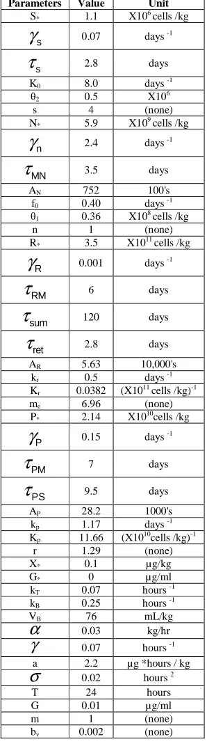
[image:9.595.224.373.205.741.2]

APPENDIX

Table A1: NORMAL STEADY STATE PARAMETERS

Parameters Value Unit S* 1.1 X106 cells /kg

s

γ

0.07 days -1

s

τ

2.8 days

K0 8.0 days -1

θ2 0.5 X106

s 4 (none)

N* 5.9 X109 cells /kg

n

γ

2.4 days -1

MN

τ

3.5 days

AN 752 100's

f0 0.40 days -1

θ1 0.36 X108 cells /kg

n 1 (none)

R* 3.5 X1011 cells /kg

R

γ

0.001 days -1

RM

τ

6 days

sum

τ

120 days

ret

τ

2.8 days

AR 5.63 10,000's

kr 0.5 days -1

Kr 0.0382 (X1011 cells /kg)-1

me 6.96 (none)

P* 2.14 X1010cells /kg

P

γ

0.15 days -1

PM

τ

7 days

PS

τ

9.5 days

AP 28.2 1000's

kp 1.17 days -1

Kp 11.66 (X1010cells /kg)-1

r 1.29 (none)

X* 0.1 µg/kg

G* 0 µg/ml

kT 0.07 hours -1

kB 0.25 hours -1

VB 76 mL/kg

α

0.03 kg/hr

γ

0.07 hours -1

a 2.2 µg *hours / kg

σ

0.02 hours 2

T 24 hours

G 0.01 µg/ml

m 1 (none)

Parameters Value Unit k 0.01 Hour-1

G

γ

0.05 Day-1

p

τ

3.27 Days

n

τ

7 Days

Acknowledgments

The authors would like to thank the referees for their helpful comments, which improved the presentation of the paper.

REFERENCES

[1]TH Price; GS Chatta; DC Dale, Blood, 1996, 88 (4), 335–340.

[2]S Basu; G Hodgson; M Katz; AR Dunn. Blood, 2002, 100 (2), 854–861.

[3]CM Kearns; WC Wang; N Stute; JN Ihle; WE Evans. J. Pediatr., 1993, 123 (2), 471–479. [4]K Mempel; T Pietsch; T Menzel; C Zeidler; K Welte, Blood, 1991, 77 (3), 1919–1922. [5]L Glass; MC Mackey, Princeton University Press, Princeton, N.J., 1988.

[6]MC Mackey; L Glass, Science, 1977,197 (1), 287–289.

[7]C Haurie; MC Mackey; DC Dale, Blood, 1998, 92 (2), 2629–2640.

[8]C Haurie; DC Dale; R Rudnicki; MC Mackey, J. Theor. Biol., 2000, 204 (3), 505–519. [9]C Haurie; R Person; DC Dale; MC Mackey, Exper. Hematol., 1999, 27 (2), 1139–1148. [10]I Roeder, Curr. Opin. Hematol., 2006, 13 (1), 222–228.

[11]T Hearn; C Haurie; MC Mackey, J. theor. Biol, 1998, 192 (3), 167–181. [12]J Belair; MC Mackey; JM Mahaffy, Math. Biosci., 1995, 128 (4), 317–346. [13]I Ostby; GKvalheim; LS Rusten; P Grottum, J. Theor. Biol., 2004, 231 (1), 69–83. [14]SI Rubinow; JL Lebowitz, J. Math. Biol., 1975, 1 (3), 187–225.

[15]A Lasota; MC Mackey, J. Math. Biol., 1984, 19 (2), 437–62.

[16]A Ducrot; V Volpert, J. Math. Model. Nat. Phenomena, 2008, 11 (2), 98–109. [17]C Foley; MC Mackey, Journal of Mathematical Biology, 2008, 58 (4), 285–322. [18]C Foley; S Bernard; MC Mackey, J. Theor. Biol., 2006, 238 (2), 754–763. [19]E Shochat; V Rom-Kedar; LA Segel, Bull. Math. Biol., 2007, 69 (3), 2299–2338. [20]S Bernard; J Belair; MC Mackey, J. Theor. Biol., 2003, 223 (4), 283–298. [21]C Colijn; C Foley; MC Mackey, Exp. Hematol., 2007, 35 (1), 898–907. [22]DC Bodensteiner; GC Doolittle, Drug Saf., 1993, 8 (2), 213–224. [23]MA Moore, Blood, 1991, 78 (3), 1–19.