BIROn - Birkbeck Institutional Research Online
Muirhead, S. and Pymar, Richard (2016) Localisation in the
Bouchaud-Anderson model. Stochastic Processes and their Applications 126 (11), pp.
3402-3462. ISSN 0304-4149.
Downloaded from:
Usage Guidelines:
Please refer to usage guidelines at
or alternatively
arXiv:1411.4032v3 [math.PR] 20 Mar 2017
STEPHEN MUIRHEAD1 AND RICHARD PYMAR2
Abstract. It is well-known that both random branching and trapping mechanisms can induce localisation phenomena in random walks; the prototypical examples being the parabolic Ander-son and Bouchaud trap models respectively. Our aim is to investigate how these localisation phenomena interact in a hybrid model combining the dynamics of the parabolic Anderson and Bouchaud trap models. Under certain natural assumptions, we show that the localisation ef-fects due to random branching and trapping mechanisms tend to (i) mutually reinforce, and (ii) induce a local correlation in the random fields (the ‘fit and stable’ hypothesis of population dynamics).
Minor revision to published version. This is an updated version of [23] containing the following minor revisions:
• A typo in the statement of Proposition 3.14 has been corrected;
• The coupling used in Section 5 has been slightly modified to fix a gap in its original statement; we thank Renato Soares dos Santos for pointing this out to us;
• A slight correction has been made to the proof of Proposition 4.11; and
• The bibliography has been updated.
1. Introduction
1.1. The Bouchaud–Anderson model. This paper studies a certain random walk model onZd
that is a hybrid of the well-knownparabolic Anderson (PAM) andBouchaud trap (BTM) models. To introduce this model, first recall the PAM, which describes the evolution of a diffusive particle in a random potential field (or, equivalently, a random branching environment; see below). Precisely, the PAM is the Cauchy problem on the latticeZd
∂u(t, z)
∂t = (∆ +ξ)u(t, z), (t, z)∈[0,∞)×Z
d; (1)
u(0, z) =1{0}(z), z∈Z
d;
whereξ={ξ(z)}z∈Zdis a collection of independent identically distributed (i.i.d.) random variables
known as the (random) potential field and ∆ is the discrete Laplacian defined by (∆f)(z) =
P
|y−z|=1(2d)−1(f(y)−f(z)), where| · |denotes the ℓ1-norm. For a large class of potential field distributions,1equation (1) has a unique non-negative solution defined for all timet. For general background information on the PAM, including its origins in the statistical physics literature and its interpretation in terms of a system of branching diffusive particles, see [13].
1Department of Mathematics, University College London (Currently: Mathematical Institute,
Uni-versity of Oxford)
2Department of Mathematics, University College London (Currently: Department of Economics,
Mathematics and Statistics - Birkbeck)
E-mail addresses:[email protected] , [email protected]. Date: March 21, 2017.
2010Mathematics Subject Classification. 60H25 (Primary) 82C44, 60F10, 60G50, 35P05 (Secondary). Key words and phrases. Parabolic Anderson model, Bouchaud trap model, localisation, intermittency. Both authors were supported by the Leverhulme Research Grant RPG-2012-608 held by Nadia Sidorova. The first author was also partial supported by the Engineering & Physical Sciences Research Council (EPSRC) Fellowship EP/M002896/1 held by Dmitry Belyaev. We would like to thank Nadia Sidorova for many invaluable suggestions, and Franziska Flegel, Onur G¨un, Renato Soares dos Santos and two anonymous referees for helpful comments.
1More specifically, those satisfying a certain integrability condition on the upper-tail; see [13].
Recall also the BTM, which describes the evolution of a diffusive particle in a random trapping landscape. Precisely, the BTM is the continuous-time Markov chain onZd defined by the jump
rates
wz→y:=
(
(2dσ(z))−1, if|y−z|= 1,
0, otherwise, (2)
where σ = {σ(z)}z∈Zd is a collection of strictly-positive i.i.d. random variables known as the
(random)trapping landscape. Remark that the density of the BTM satisfies the equation
∂u(t, z)
∂t = ∆σ
−1u(t, z), (t, z)∈[0,∞)×Zd, (3)
where, for clarity, we stress that the operator ∆σ−1 acts as
(∆σ−1f)(z) = X
|y−z|=1
(2dσ(y))−1f(y)−σ−1(z)f(z).
For general background information on the BTM, including its origins in the study of spin-glasses dynamics and its broad utility as a simple model for a variety of trapping behaviour, see [4].
The PAM and BTM are of great interest in the theory of random processes because they exhibitintermittency, that is, unlike other commonly studied models of diffusion, their long-term behaviour cannot, in general, be described with a simple averaging principle (see [13] and [4] for a general overview of the PAM and BTM respectively.) Instead, extremes in the respective random environments may create concentration effects, which can result in the eventuallocalisation of the solution to equations (1) and (3) respectively over long periods of time. In the most extreme cases, the solution localises on just a few sites.
Our aim is to study how the localisation phenomena in the PAM and the BTM interact. To do this, we consider the Cauchy problem on the latticeZd
∂u(t, z)
∂t = (∆σ
−1+ξ)u(t, z), (t, z)∈[0,∞)×Zd; (4)
u(0, z) =1{0}(z), z∈Z
d;
derived by replacing the discrete Laplacian in equation (1) with the generator of the BTM in equation (3). We refer to equation (4) as theBouchaud–Anderson model (BAM).
By analogy with the PAM (see [13], Section 1.2), the solution to equation (4) has a natural interpretation as the expected number of particles in a system of continuously-branching diffusive particles on the latticeZd specified by:
• Initialisation: A single particle at the origin;
• Branching: The local branching rate for a particle at a sitez is given byξ(z);
• Trapping: Each particle evolves as an independent BTM, that is, the waiting time at each visit to a site z is independent and distributed exponentially with mean σ(z), with the subsequent site chosen uniformly from among the nearest neighbours.
This interpretation can be formalised in the Feynman-Kac representation of the solution to (4):
u(t, z) :=E0
exp
Z t
0
ξ(Xs)ds)
1{X
t=z}
, (5)
whereX is the BTM and, forz∈Zd,Ez denotes the expectation overX given thatX0=z. As
we shall see, the interaction between the random branching and trapping mechanisms makes the localisation behaviour of the BAM highly non-trivial.
1.2. Localisation in the PAM and BTM. The PAM and BTM are said tolocaliseif, ast→ ∞, the solution of equations (1) and (3) respectively are eventually concentrated on a small number of sites with overwhelming probability, i.e. if there exists a (random)localisation set Γtsuch that, ast→ ∞,|Γt|=to(1) and
P
z∈Γtu(t, z)
whereU(t) :=P
z∈Zdu(t, z) is the total mass of the solution (in the BTM, this is identically one);
see Section 1.8 for the definition of the asymptotic notation used here and throughout the paper. Naturally, the primary measure of the strength of localisation in the PAM and BTM is the cardinality of the localisation set Γt. As such, the most extreme form of localisation iscomplete localisation, which occurs if the total mass is eventually concentrated at just one site, i.e. if Γt can be chosen in equation (6) such that|Γt|= 1. A finer measure of the strength of localisation is the radius of influence, which measures the extent to which localisation sites themselves are determined by purely local features of the random environment. More precisely, the radius of influenceρis the smallest integer for which the localisation sites can be determined by maximising a functional onZd that depends on the random environments only through their values in balls
of radiusρaround each site.
Broadly speaking, localisation in the PAM and BTM is generated by the structure-forming effects of extremes in the respective random environment. If these extremes are both sufficiently pronounced and sufficiently regular, over long periods of time the model will come to adopt the structure present in the environment, with localisation the most extreme manifestation of this. Naturally then, the strength of localisation in the PAM and BTM should depend on (i) the asymptotic rate of decay, and (ii) the regularity of the upper-tail of the random variables ξ(0) andσ(0). In this context, it is convenient to restrictξ(0) andσ(0) to be strictly-positive and to characterise these random variables by their exponential tail decay ratefunction
gξ(x) :=−log(P(ξ(0)> x)) and gσ(x) :=−log(P(σ(0)> x))
for then (i) and (ii) translate to the asymptotic growth and regularity of the non-decreasing functionsgξ andgσ.
We briefly outline some known results on localisation in the PAM and BTM. For simplicity, we shall assume all necessary regularity conditions without further specification.
1.2.1. Localisation in the parabolic Anderson model. The conditions under which the PAM com-pletely localises in the sense of equation (6) has been the subject of intense and ongoing research over the last 25 years. The current understanding is that double-exponential tail decay (gξ(x)≈ex) forms the boundary of the complete localisation universality class. More precisely, it is conjec-tured that the PAM exhibits complete localisation as long as loggξ(x)≪x. This has been proven (in [20]) in the extremal2 case of Pareto-like tail decay (gξ(x) ∼ γlogx, for γ > d), and more recently (in [26] and [10]) in the case of Weibull-like tail decay (gξ(x)∼xγ). On the other hand, if loggξ(x) ≫ x, then complete localisation is known not to hold (see [12]). What occurs in the interface regime of double-exponential tail decay (loggξ(x)∼cx, for c > 0) is not currently well-understood.
As for the radius of influence of the potential field,ρPAM, in the case of Pareto-like tail decay it has been shown (see [20]) that ρPAM = 0, in other words, the localisation site can be deter-mined by maximising a functional that depends on the potential fieldξonly through its value at individual lattice sites, with interactions between neighbouring lattice sites having no influence on localisation. On the other hand, in the case of Weibull-like tail decay (gξ(x) ∼xγ), the radius of influence has been shown (see [10]) to be ρPAM= [(γ−1)/2]+, where [x] and x+ denote the integer and positive parts of x respectively. Clearly this implies that ρPAM = 0 if and only if
γ <3, and also thatρPAM→ ∞in theγ→ ∞limit.
1.2.2. Localisation in the Bouchaud trap model. The study of localisation in the Bouchaud trap model has also received considerable attention over the last 10 years. A notable feature of the BTM is that localisation can only occur in dimension one. In higher dimensions, the traps either have negligible effect in the limit (if the tail is integrable, by virtue of the law of large numbers), or are visited in such a way that their overall effect is spatially-homogeneous (see [11] and [4] for a proof of this result in the case of Pareto-like tail decay, although the result is thought to hold more generally for arbitrary non-integrable tail decay).
2This case is extremal in the sense that ifg
ξ(x)∼γlogxforγ > dorγ=d= 1 then the solution to equation (1)
On the other hand, it is known that in dimension one, Pareto-like tail decay (gσ(x)∼clogx,
c >0) forms the boundary of the localisation universality class. More precisely, if logx=O(gσ(x)), it is known that the BTM does not localise in the sense of equation (6) (although it does localise in a certain weaker sense; see, e.g. [11]). On the other hand, it was proven in [22] that for sub-Pareto tail decay (gσ(x)≪logx), the BTM localises on exactly two-sites in the limit, with a radius of influence (i.e. of the trapping landscape) equal to 0.
1.3. Overview of our results. Before detailing our results in full, we first provide a brief overview to highlight salient features; this section is for exposition only, and is not intended to be mathematically rigorous. A complete description of our results follows in Section 1.7 below. In this initial study of localisation in the BAM, we focus on the case where both potential distributionξ(0) and trap distributionσ(0) have Weibull tail decay
P(ξ(0)> x) =e−xγ and P(σ(0)> x) =e−xµ γ, µ >0.
Our results also hold in theγ, µ→0 limit (with some caveats; see Section 1.6). As we shall see, the BAM with Weibull tail decay turns out to be a natural regime to study, since the interaction between the potential field and trapping landscape exhibits certain phase transitions in (γ, µ).
1.3.1. Complete localisation. Our first main result establishes the complete localisation of the BAM across the entire regime (see Theorem 1.7 below).
Theorem 1.1. There exists a (random) site Ztsuch that, as t→ ∞,
u(t, Zt)
U(t) →1 in probability.
That the BAM completely localises for some (γ, µ) is expected, since the PAM with Weibull potential also exhibits complete localisation. More surprising, however, is that complete localisa-tion occurs regardless of the presence of very large traps, even in dimension one, sincea priori it might be thought that large traps would draw probability mass away from the localisation site.
1.3.2. Mutual reinforcement of localisation effects due to the PAM and the BTM. Since complete localisation holds in the entire regime, in order to probe the interaction between the potential field and trapping landscape we need a finer measure of localisation. Such a measure is provided by the
radius of influence ρ, which as described above is the smallest integer for which the localisation siteZtcan be determined by maximising a functional onZdthat depends onξandσonly through their values in balls of radiusρaround each site. Our second main result is to determine the radius of influenceρ, and to prove its optimality (see Theorem 1.7 and part (a) of Theorem 1.10 below).
Theorem 1.2. The radius of influence is
ρ:=
γ−1
2
µ µ+ 1+
1 2
+
.
Note that ρis a decreasing function of the strength of both the potential field and trapping landscape (i.e. an increasing function of γ andµ), in other words, the localisation effects due to the PAM and BTM aremutually reinforcing.
1 2 3 4 5 2
4 6
[image:6.612.203.400.98.263.2]γ µ
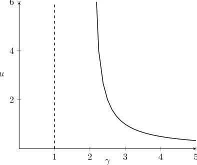
Figure 1. Partition of the parameter space of the BAM according to the whether the BAM is ‘strongly reducible’ to the PAM with the usual potentialξ(left of the dashed line) or ‘weakly reducible’ to the PAM with the potential replaced with the ‘net growth rate’ η (left of the bold curve). The boundary curve is µ = 1/(γ−2).
Theorem 1.3. The BAM is strongly reducible to the PAM if and only if γ < 1. The BAM is weakly reducible to the PAM if and only if ρ= 0andγ≥1.
1.3.4. Local correlation between the potential field and trapping landscape: The ‘fit and stable’ hypothesis. Our final result is to establish the local correlation between the potential field and trapping landscape (where ‘local’ is from the perspective of the localisation site); this is the so-called ‘fit and stable’ hypothesis that has been predicted numerically in the mathematical biology literature (see, e.g., [6]), but never rigorously confirmed (see Section 1.5 below). Interestingly, the correlation that we observe is positive at the localisation site, but negative away from the localisation site, providing an unexpected extension to the ‘fit and stable’ hypothesis.
To describe this correlation, we shall need to define a second, possibly smaller, radius of influence
ρξ :=
γ−1
2
µ µ+ 1
+
∈ {ρ−1, ρ},
which is the the smallest integer for which the localisation siteZt can be determined by a max-imising a functional onZd that depends onξonly through its values in balls of radius ρξ around
each site (note, the functional must still depend on σ through balls of radius at least ρ). For simplicity, we exclude here the ‘interface cases’, i.e. the points of discontinuity ofρξ.
Theorem 1.4. Assume thatγ≥1, so that the BAM is not strongly reducible to the PAM. LetZt
denote the site of complete localisation. Then, ast→ ∞eventually almost surely: (i) the random variables ξ(Zt)andσ(Zt)are positively correlated; and (ii) for all z such that 0<|z−Zt| ≤ρξ,
the random variablesξ(z)andσ(z)are negatively correlated.
In Theorem 1.9 below we make explicit the nature of this correlation, as well as providing a full description of the localisation site, determining its asymptotic distance from the origin, the local profile of the potential field and trapping landscape, and its ageing behaviour.
First, proving localisation in the BAM requires the development of the spectral theory of op-erators of the form ∆σ−1+ξ, including path expansions and Feynman-Kac representations for the principal eigenvalue and eigenfunction respectively. To our knowledge this theory has not appeared in the literature before, and may be of independent interest, including in the study of position-dependent mass Schr¨odinger operators (see Section 1.5 below). In the particular case of the BAM with Weibull tails, we also extend existing techniques to establish the max-class of local eigenvalues; this is necessary in order to extract extra information about the local correlation in the potential field and trapping landscape.
Second, in order to analyse the ‘screening effect’ of heavy traps, standard percolation estimates are insufficient: in dimension one, because of the geometry; in dimensions higher than one, because of complex dependencies between the potential field, the trapping landscape, and the localisation siteZt. In dimension one we analyse heavy traps using coarse graining methods; in higher dimen-sions, we implement new ideas that allow us to apply percolation estimates in the presence of the dependencies.
In addition, our methods provide a new approach to working with ‘cluster expansions’. Al-though these expansions have appeared in the literature before (see, e.g., [1, 10]), the standard approach has been to access them via resolvent formalism. Our techniques provides a purely probabilistic approach to ‘cluster expansion’, which avoids many of the technicalities of the resol-vent formalism. One application would be a simpler, purely probabilistic proof of the localisation results on the PAM found in [10].
1.5. Connections to the literature. Although this is the first work to consider the BAM, there are clear connections between the BAM and other models in the literature. First, the BAM can be interpreted as the thermodynamic limit of a particle system with random branching and trapping mechanisms (given, respectively, by the potential fieldξand the trapping landscapeσ). In the probability literature there have been several other analyses of models combining random branching and trapping mechanisms – in particular, trapping mechanisms given by asymmetric transition probabilities [3] and random conductances [28] – although these have not considered the localisation properties of the model, focusing instead on the growth of the total population.
Similar models have also appeared in the mathematical biological literature, where they find an application in the study of population dynamics. Here the branching and trapping rates are recast as the fitness (‘adaptedness’) and stability (‘adaptability’) respectively of individual states (e.g. geographic locations, genetic configurations etc.). While the literature contains several models which allow for randomness in either the fitness [19, 24] or stability [18, 21, 27], most relevant is [6] which considers a model in whichboth these characteristics vary. Indeed, the model considered in [6] is essentially identical to the BAM, except it is defined in a domain without any geometry: when an individual’s state changes, the fitness and stability are re-sampled according to their respective distributions.3 The primary observation in [6] (obtained numerically) is the tendency of populations to concentrate on states which are both fit and stable: the ‘fit and stable’ hypothesis. Our results provide the first rigorous analysis of this phenomenon. Indeed, our results actually suggest a refinement of the hypothesis (for our model with geometry): that populations concentrate on states which are fit and stable,but also for which neighbouring states are both fit andunstable.
Second, operators of the form ∆σ−1+ξ have important applications in quantum mechanics, since their eigenvalues give the energy levels of a particle whose effective mass is position-dependent (see, e.g., [7, 8, 25]). To make the connection, consider the position-dependent mass Schr¨odinger equation for a particle with effective massσin a potential fieldξ. This equation has a Hamiltonian of general form (see [25])
1 2 σ
−α∇σ−β∇σ−γ+σ−γ∇σ−β∇σ−α
+ξ , α, β, γ≥0, α+β+γ= 1.
3A second minor difference is that the population size is kept constant by the deletion of a uniformly chosen
Although there is no canonical choice for α, β, γ, in the discrete setting a natural restriction is
β= 0, which avoids symmetry breaking in the definition of∇. Specialising to the caseα=γ= 1/2 gives the Hamiltonian
σ−1
2∆σ−12 +ξ=σ−21 ∆σ−1+ξσ12. (7)
We remark that the Hamiltonian in (7) is the ‘symmetrised’ form of the operator ∆σ−1+ξ, and hence has equivalent spectral theory. In Section 3 we develop general theory for operators of the form ∆σ−1+ξ, including deriving path expansions and Feynman-Kac representations for the principal eigenvalue and eigenfunction respectively. This section is entirely self-contained, and is completely deterministic, and we expect that it will be of independent interest.
Third, there are connections between the BAM and the PAM in the case where the potential field distribution ξ(0) is allowed to take on highly negative (or even infinitely negative) values, which may be interpreted as ‘traps’. Previous work has noted the minimal influence of such ‘traps’ in d≥2 (see, e.g. [13, Section 2.4]), essentially due to percolation estimates, an observation that finds echoes in our results and methods. However, there are clear differences between this model and the BAM, primarily due to the fact that the traps in the BAM may coexist with sites of high potential; this coexistence underlies the phenomena of mutual reinforcement and correlation that we observe in the BAM. On the other hand, in dimension one the effect of highly negative potential values in the PAM is significant (see [5]). Indeed, since such sites cannot be avoided, their effect is to ‘screen’ off the growth that would otherwise occur from sites of high potential, and so the asymptotic growth of the solution depends heavily on the relationship between the upper and lower tails ofξ(0). Again, this is reminiscent of our results in dimension one, which are only valid if the trap distribution decays sufficiently fast to ensure ‘screening’ effects are negligible.
1.6. The formal set-up for the paper. For the rest of the paper, we make the following assumptions on the potential fieldξand the trapping landscapeσ:
Assumption 1.5 (Assumption on the potential field distribution). The random variable ξ(0) is strictly-positive and satisfies
¯
Fξ(x) =e−x
γ
,
for someγ >0, whereF¯ξ(x) := 1−Fξ(x) :=P(ξ(0)> x).
Assumption 1.6 (Assumptions on the trap distribution). The random variable σ(0)satisfies:
(a) No quick sites: The quantity
δσ:= essinfσ(0)
is strictly positive;
(b) Regularity: The quantity
µ:= lim x→∞
loggσ(x) logx
exists and is finite. Ifµ >0, thenσ(0)has a continuous density functionfσ(x)with a Weibull upper-tail, i.e. for sufficiently largex,
¯
Fσ(x) = exp{−xµ},
where F¯σ(x) := 1−Fσ(x) := P(σ(0) > x). If µ = 0, then σ(0) has a continuous density
functionfσ(x), with the property that
fσ(ax)∼fσ(bx)
for any ax, bx→ ∞ such thatax∼bx (see Section 1.8 for the asymptotic notation). In both
cases, the lower-tail offσ satisfies, asx→0,
fσ(x+δσ) =o(e−1/x).
(c) Sufficiently fast tail decay: Asx→ ∞ eventually, for someε >0,
gσ(x)>(1 +ε) log logx;
(d) Regularity: There exists ac∈(1,∞]such that
lim x→∞
gσ(x) log logx =c ,
with the convergence eventually monotone in the casec=∞.
We wish to briefly comment on the nature of the above assumptions onξ(0) and σ(0). First, we claim that the BAM with Weibull potential field is a natural regime in which to observe the interaction between the localisation effects in the PAM and the BTM. If the potential field is any stronger (indeed if γ < 1), the BAM is strongly reducible to the PAM4. On the other hand, if the potential field is any weaker, the effect of the trapping landscape, while present, is harder to measure. To see why, recall that the PAM with Weibull potential field has been shown to completely localise with a certain finite radius of influence ρPAM; it is on the level of this radius that we measure the impact of the trapping landscapeσ. SinceρPAM→ ∞in theγ → ∞limit, the effect of changes toρPAM become harder to quantify, and we leave this study to future work. Second, the regularity assumption onξ(0) is imposed mainly for simplicity; weaker regularity assumptions (like those found in [1] and [2] for instance) are possible, although they introduce certain technical difficulties that we wish to avoid. Finally, note that equivalent results for the BAM with Pareto-like potential field can be naturally deduced by considering our results in the
γ→0 limit.
Turning to the assumptions on σ(0), first note that the quantity µ measures the ‘Weibull-ness’ of the upper-tail of σ(0), with the case µ = 0 corresponding to a stronger-than-Weibull trapping landscape. For simplicity, we have chosen not to consider weaker-than-Weibull trapping landscapes in this paper; equivalent results can be naturally deduced by considering our results in theµ→ ∞limit. As with ξ(0), the regularity assumptions onσ(0) are certainly not optimal for our results to hold; they are chosen mainly for simplicity. On the other hand, our assumption that
σ(0) is bounded away from zero is essential. Indeed we expect that the nature of the localisation behaviour will change if ‘quick’ sites are present. Finally, the additional tail decay assumption in dimension one is also essential, and our results and methods break down completely without it. Note, however, that this condition is only violated for trap distributions with extremely heavy tails, such as ifσ(0) is alog-Pareto random variable.
1.7. Full description of our results. Here we describe our results in full, expanding on the exposition given in Section 1.3. In order to state our results explicitly, we shall need to intro-duce some notation. Recall the parameterµ ∈[0,∞) from Assumption 1.6, which describes the ‘Weibull-like’ decay parameter of the upper-tail ofσ(0). Recall also from Section 1.3 the radius of influence
ρ:=
γ−1
2
µ µ+ 1 +
1 2
+
and the, possibly smaller, radius of influence of the potential fieldξ,
ρξ :=
γ−1 2
µ µ+ 1
+
∈ {ρ−1, ρ} ≤ρ .
The relationship between ρand ρξ is depicted in Figure 2; we defer further discussion onρand
ρξ to Remark 1.11.
Next we describe explicitly the localisation site. For each z ∈ Zd and n∈ N, define the ball
B(z, n) :={y ∈Zd :|y−z| ≤n}. For eachz∈Zd, define the Hamiltonian H(z) := ∆σ−1+ξ1B(z,ρ
ξ)
4Note however that, because of Assumption 1.6, this conclusion does not apply in dimension one if the trapping
2 4 6 8 10 2
4 6 8 10
γ µ
ρ, ρξ= 0
ρ= 1 ρ= 2
ρ= 3
[image:10.612.194.410.98.275.2]ρξ= 1 ρξ= 2 ρξ= 3
Figure 2. Partition of the parameter space of the BAM according to the values of ρ (bold lines) and ρξ (dashed lines). The boundary curves are of the form
µ= (2i−1)/(γ−2i) andµ= (2i)/(γ−2i−1), for i∈N\ {0}.
restricted to the domainB(z, ρ) with Dirichlet boundary conditions, denoting byλ(z) its principal eigenvalue. Note that each λ(z) is real since the Hamiltonian H(z) is similar to the Hermitian operator
σ−12H(z)σ12 =σ−12∆σ−12 +ξ
1B(z,ρ
ξ).
We refer toλ(z) as thelocal principal eigenvalue atz, and remark that it is a certain functional of the sets ξ(ρξ)(z) := {ξ(y)}
y∈B(z,ρξ) and σ
(ρ)(z) := {σ(y)}
y∈B(z,ρ). Note that the random
variables{λ(z)}z∈Zdare identically distributed, and have a dependency range bounded by 2ρ, i.e.
the random variablesλ(y) andλ(z) are independent if and only if|y−z|>2ρ. Remark also that in the special caseρ= 0, λ(z) reduces to the ‘net growth rate’η(z) =ξ(z)−σ−1(z).
For any sufficiently larget, define apenalisation functional Ψt:Zd→Rby
Ψt(z) :=λ(z)−|z|
γt log logt .
Note that Ψthas a similar form to the penalisation functional introduced in [10] to prove complete localisation in the PAM with Weibull potential field, representing the trade-off between energetic forces (given by the local principal eigenvalueλ(z)) and entropic forces (given by a probabilistic penalty which is linear in|z|and decaying int); see Remark 1.8.
Define a large ‘macrobox’ Vt := [−Rt, Rt]d ∩Zd, with Rt := t(logt)
1
γ. Fix a constant 0 <
θ < 1/2 and define the macrobox level Lt := ((1−θ) log|Vt|)
1
γ. Let the subset Π(Lt) :=
z∈Zd :ξ(z)> Lt ∩Vtconsist of sites inVtat whichξ-exceedances of the levelLtoccur. Finally, define the random site
Zt:= arg max z∈Π(Lt)
Ψt(z).
The siteZtis well-defined eventually almost surely since, as we show in Lemma 4.1, the set Π(Lt) is non-empty and finite eventually almost surely. Moreover, for t sufficiently large, Zt almost surely does not depend on the particular choice of θ. We present again (see Theorem 1.1) our main theorem:
Theorem 1.7 (Complete localisation). As t→ ∞,
u(t, Zt)
Remark 1.8. In order to determineZt explicitly, a finite approximation is available forλ(z) (see Proposition 5.1 for a precise formulation):
λ(z)≈η(z) +σ−1(z) X
2≤k≤2j
X
p∈Γk(z,z)
pi6=z,0<i<k
Set(p)⊆B(z,ρ)
Y
0<i<k
(2d)−1 σ−1(pi)
λ(z)−ηz(pi), (8)
where j := [γ−1] and ηz := ξ1B(z,ρ
ξ)−σ
−1; see Section 1.8 for the definition of the path set Γk(z, z). This path expansion can be iteratively evaluated to approximate Ψt(z) as an explicit function ofξ(ρξ)(z), σ(ρ)(z),|z|and t, which, as we show, is sufficiently precise to determine the
localisation siteZt with overwhelming probability.
Before stating our second and third main results we shall introduce some more notation. First we define exponents that explicitly describe the correlation of the fieldsξandσaround the localisation site Zt. To this end, define the functionqξ :N→[0,1] and the non-negative constantqσ by
qξ(x) :=
1− 2x γ−1−
1 µ+1
+
ifγ >1,
(1−x)+ else,
and qσ:=
γ−1
µ+ 1
+
.
We shall also need the concept of ‘interface cases’, which correspond to the values of (γ, µ) whereρ, and respectivelyρξ, are transitioning from one integer to the next. To this end define the sets
B:=
(γ, µ) : γ−1 2
µ µ+ 1 +
1 2 =ρ
and Bξ :=
(γ, µ) : γ−1 2
µ µ+ 1 =ρξ
.
Note that these sets correspond, respectively, to the bold and dashed curves in Figure 2. Finally, define the random timeTt:= inf{s >0 :Zt+s6=Zt} and the scales
rt:= t(dlogt)
1 γ−1
log logt and at:= (dlogt)
1
γ. (9)
The scalesrt andat describe, respectively, the scale of the distance from the origin of the locali-sation site and the scale of the height of the potential field at the localilocali-sation site.
Theorem 1.9 (Description of the localisation site). Ast→ ∞the following hold: (a) (Localisation distance)
Zt
rt
⇒X in law,
where X is a random vector whose coordinates are independent and distributed as Laplace (two-sided exponential) random variables with absolute-moment one.
(b) (Local correlation of the potential field) If (γ, µ)∈ B/ ξ, then for eachz∈B(0, ρξ)there exists
ac >0 such that
ξ(Zt+z)
aqξ(|z|)
t
→c in probability. (10)
If (γ, µ)∈ Bξ, then (10) holds for each z∈B(0, ρξ −1), and moreover, for each z such that
|z|=ρξ there exists ac >0such that,
fξ(Zt+z)(x)→
ecxfξ(x)
E[ecξ(0)],
uniformly over x ∈ (0, Lt), where fξ(z) is the density of the potential field at site z (see
Assumption 1.5).
(c) (Correlation of the trapping landscape at Zt) If µ > 0 and γ >1, then there exists a c > 0
such that
σ(Zt)
aqσ
t
Ifµ= 0 andγ >1 then, for each ν >0,
P
logσ(Zt)
logat
> qσ−ν
→1.
Ifγ= 1 then,
fσ(Zt)(x)→
e−1/xfσ(x)
E[e−1/σ(0)] ,
uniformly overx, wherefσ(Zt) is the density of the trapping landscape at siteZt.
(d) (Local correlation of the trapping landscape) If(γ, µ)∈ B, then for each/ z∈B(0, ρ)\ {0}
σ(Zt+z)→δσ in probability. (11)
If (γ, µ)∈ B, then (11) holds for eachz ∈ B(0, ρ)\ {0} and moreover, for each z such that |z|=ρ, there exists ac >0such that
fσ(Zt+z)(x)→
ec/xfσ(x)
E[ec/σ(0)],
uniformly overx, where fσ(z) is the density of the trapping landscape at site z (see
Assump-tion 1.6). (e) (Ageing)
Tt
t ⇒Θ in law,
whereΘis a non-degenerate almost surely positive random variable.
Theorem 1.10(Optimality results). As t→ ∞ the following hold:
(a) (Optimality of the radius of influence) The radius of influence ρ is optimal, in other words, there does not exist a functionalψt, depending on ξ andσ only through their values in balls
of radiusρ−1 around each site z, such that
P
Zt= arg max z∈Zd
ψt(z)
→1. (12)
(b) (Optimality of the radius of influence with respect to the potential field) The radius of influ-ence of the potential field ρξ is optimal, in other words, there does not exist a functionalψt,
depending on ξonly through its values in balls of radiusρξ−1 around each sitez, such that
P
Zt= arg max z∈Zd
ψt(z)
→1. (13)
(c) (Criterion for reduction to the potentialξ) The localisation site is independent of the trapping landscapeσ if and only if γ <1, in other words, if and only ifγ <1, there exists a random sitezt∈Zd, independent ofσ, such that,
P(Zt=zt)→1. (14)
(d) (Criterion for reduction to the ‘net growth rate’ η) The localisation site Zt depends onξ and
σonly through the value ofη if and only ifρ= 0, in other words, if and only if ρ= 0, there exists a random sitezt∈Zd, dependent onξ andσonly through η, such that,
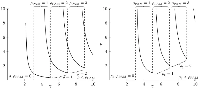
P(Zt=zt)→1. (15) Remark 1.11. We note several interesting features of the radius of influenceρ. As remarked above,
2 4 6 8 10 2
4 6 8 10
γ µ
ρ, ρPAM= 0 ρ= 1 ρρ < ρ= 2PAM
ρPAM= 1ρPAM= 2ρPAM= 3
2 4 6 8 10
2 4 6 8 10
γ µ
ρξ, ρPAM= 0 ρξ= 1
ρξ= 2
ρPAM= 1 ρPAM= 2ρPAM= 3
[image:13.612.99.508.94.275.2]ρξ< ρPAM
Figure 3. Partition of the parameter space of the BAM according to the rela-tionship betweenρ(bold lines) and ρPAM (dashed lines), andρξ (bold lines) and
ρPAM(dashed lines) respectively, where ρPAM denotes the radius of influence in the equivalent PAM with identical potential field. The boundary curves are of the formµ= (2i−1)/(γ−2i) andµ= (2i)/(γ−2i−1) respectively, fori∈N\{0}.
Remark 1.12. The shape of the local profile of the potential field and trapping landscape in parts (b)–(d) of Theorem 1.9 is derived by considering the path expansion in equation (8) and determin-ing the values ofξandσthat appropriately balance: (i) the increase inλgained from favourable realisations ofξandσ; and (ii) the probabilistic penalty that results from such favourable realisa-tions ofξandσif they are too unlikely. This balance is expressed through a convex function whose integral is asymptotically concentrated in the regions specified in Theorem 1.9. This computation is carried out in the proof of Proposition 5.3, identifying the constants in Theorem 1.9 explicitly. We also give some heuristic reasons why we must distinguish the cases (γ, µ) ∈ B,Bξ in the correlation results. If (γ, µ)∈ B/ ξ, then the value ofξ(Zt+z) is growing (with high probability) as
t→ ∞for eachz∈B(0, ρξ). However, if (γ, µ)∈ Bξ, this only occurs for z∈B(0, ρξ−1); at the interface of the radius, where|z|=ρξ, the value ofξ(Zt+z) instead converges to a certain random variable with law distinct from the law ofξ(0). Similarly, for (γ, µ)∈ B/ ,σ(Zt+z) converges toδσ for eachz∈B(0, ρ)\ {0}. However, if (γ, µ)∈ B, then this is only true for z∈B(0, ρ−1)\ {0}. If|z|=ρ, the value ofσ(Zt+z) instead converges to a certain random variable with law distinct from the law of σ(0). These properties are reflective of the fact that the correlation in the fields
ξandσinduced by the localisation site Ztdecays away from the site.
We also explain why the cases γ ≤1 and µ= 0 must be further distinguished in our profile forσ(Zt). If γ >1 then the value of σ(Zt) is growing, and indeed growing with a deterministic leading order. However, ifγ = 1, this is no longer true and insteadσ(Zt) converges to a certain random variable with law distinct from the law ofσ(0).5 The caseµ= 0 must be distinguished for a different reason; in this case, the extremes ofσare so large that there are many sites z for whichσ−1(z) is smaller than the gap in the top statistics of Ψt. Past this threshold, differences in the magnitude of σ no longer materially influence the determination of Zt, and so we lose a degree of certainty about the order of growth ofσ(Zt).
Note finally that if (γ, µ) is not inB andBξ respectively, then the probabilities in equations (12) and (13) actually converge to 0 for any such ψt; otherwise, the respective probability will converge to a constantc ∈ (0,1). Similarly, if (γ, µ) lies to the right of the dashed or bold line in Figure 1, the probabilities in (14) and (15) respectively converge to 0 for any suchzt; if (γ, µ)
5Of course, in the caseγ <1, with overwhelming probability σis independent of the localisation siteZ
t (cf.
lies on either line, the repective probability instead converges to a constantc∈(0,1). We do not prove these additional results here.
1.8. Notation. Here we list notation that will be commonly used for the remainder of the paper.
Asymptotic notation: For functionsf and gwe usef ∼gto denote that
lim
x→∞f(x)/g(x) = 1,
andf =o(g) orf ≪gto denote that
lim
x→∞f(x)/g(x) = 0.
We usef =O(g) to denote that, asx→ ∞, eventually for some constantc >0,
|f(x)|< c|g(x)|.
Notation for paths: For an integerk and sites y, z∈ Zd, let Γk(y, z) be the set of nearest
neighbour paths inZd of lengthkrunning fromy toz, with eachp∈Γk(y, z) indexed as
y=:p0→p1→p2→. . .→pk:=z .
Similarly, denote
Γk(y) := [ z∈Zd
Γk(y, z), Γ(y, z) := [ k∈N
Γk(y, z),
Γ(y) := [ k∈N
Γk(y), Γ := [ y∈Zd
Γ(y).
For a sitez∈Zd, letn(z) denote the number of shortest paths from the origin toz, i.e.
n(z) :=|Γ|z|(0, z)|.
For a path p∈Γk(y, z) denote Set(p) := {p0, p1, . . . , pk} and |p| :=k. For a nearest neighbour random walk X let p(Xt)∈ Γ(X0) denote the geometric path associated with the trajectory of
{Xs}s≤t and let pk(X) ∈ Γk(X0) denote the geometric path associated with the random walk
{Xs}s≥0up to and including itskth jump.
Notation for sets: For a domainD∈Zd, denote by
∂D={y∈Dc: there existsx∈D such that|x−y|= 1}.
For a setS∈Zd defineB(S, n) :=S
z∈SB(z, n) and sep (S) := minx6=y∈S{|x−y|}.
Notation for solutions of the BAM: For eachy, z∈Zddefineuy(t, z) to be the solution of
the Cauchy problem
∂uy(t, z)
∂t = (∆σ
−1+ξ)uy(t, z), (t, z)∈[0,∞)×Zd;
uy(0, z) =1{y}(z), z∈Z
d;
and, forz∈Zd andp∈Γ, define
up(t, z) :=E p0
exp
Z t
0
ξ(Xs)ds
1{X
t=z}1{p(X
t)=p}
, Up(t) := X
z∈Zd
up(t, z).
Notation for local principal eigenvalues: For eachz ∈Zd and n∈ N define then-local
principal eigenvalueλ(n)(z) to be the principal eigenvalue of the Hamiltonian
H(n)(z) := ∆σ−1+ξ
restricted to the domainB(z, n) with Dirichlet boundary conditions.
2. Outline of proof
The main idea of the proof of Theorem 1.7 is that the solution u(t, z) can be decomposed into disjoint components by reference to the trajectories of the underlying BTM in the Feynman-Kac representation in (5). Using such a path decomposition, we prove complete localisation by establishing that: (i) a single component carries the entire non-negligible part of the solution; and (ii) the non-negligible component is localised atZt.
To assist in the proof, we introduce the scale
dt:= 1
γ(dlogt)
1
γ−1 (16)
which is the derivative (on the log scale) of the height scaleat, and naturally examines the gaps in the maximisers ofξin growing boxes. We also introduce auxiliary scaling functionsft, ht, et, bt→0 and gt, st → ∞ as t → ∞ that are convenient placeholders for negligibly decaying (respectively growing) functions. For technical reasons, we shall need to choose these functions to satisfy certain relationships, as follows. First, letstbe such that
(logst)2≪log logt .
Then, chooseft, ht, et, btandgtsatisfying
max{F¯σ(st),(logst)2/log logt,1/log logst}gt≪bt≪ftht≪gtht≪et. (17) It is easy to check that such a choice is always possible.
Path decomposition. We explain here how to construct the path decomposition. Recall the defi-nition ofVtfrom Section 1.7. For a pathp∈Γ(0) such that Set(p)⊆Vt, let
z(p):= arg max z∈Set(p)
λ(z)
which is well-defined almost surely. Abbreviate
Bt:=B(0,|Zt|(1 +ht))∩Vt.
We partition the path set Γ(0) into the following five disjoint components
Ei t:=
p∈Γ(0) : Set(p)⊆Bt, z(p)=Zt , i= 1 ; (non-negligible component)
p∈Γ(0) : Set(p)⊆Vt, z(p)∈Π(Lt)\Zt , i= 2 ; (path does not hit best site)
p∈Γ(0) : Set(p)⊆Vt,Set(p)6⊆Bt, z(p)=Zt , i= 3 ; (path travels far)
p∈Γ(0) : Set(p)⊆Vt, z(p)∈/Π(Lt) , i= 4 ; (path avoids all high sites)
{p∈Γ(0) : Set(p)6⊆Vt}, i= 5 ; (path leaves macrobox)
and associate each component Ei
t with a portion of the total mass U(t) of the solution. As such, for each 1≤i≤5, let
ui(t, z) := X
p∈Ei t
up(t, z) and Ui(t) = X
z∈Zd
ui(t, z).
Our strategy is to establish that each ofU2(t),U3(t),U4(t) andU5(t) are negligible with respect to the total massU(t) of the solution, in other words that,
Ui(t)
U(t) →0 in probability, fori= 2,3,4,5.
To complete the proof of localisation, we also prove thatU1(t) is localised atZt, i.e. that,
u1(t, Zt)
U1(t) →1 in probability.
Note that this strategy requires a balance to be struck in how Bt is defined; it must be large enough that U3(t) is negligible, but small enough to ensure localisation. The scale h
Negligible paths. The negligibility ofU4(t) andU5(t) are simple to establish; the main difficulty is establishing the negligibility ofU2(t) andU3(t). Our proof is based on formalising two heuristics.
First heuristic: Recall the constant j := [γ−1]≥ρand the definition of thej-local principal eigenvalueλ(j) from Section 1.8. We expect that, for a pathp∈Γ(0)\E5
t,
Up(t)≈expntλ(j)(z(p))oa−|t p| , (18) which represents the balance between (i) the exponential growth of the solution at each site, and (ii) the probabilistic penalty for travelling each step along the pathp.
The accuracy of this heuristic relies on some subtle observations about the BAM (and indeed the PAM) which we shall briefly discuss further. First is the claim that the j-local principal eigenvalues closely approximate the exponential growth rate of the solution at a site (note that here we could take a slightly smaller constant in place ofj, but j will turn out to be convenient for another reason; see immediately below). This approximation, in turn, is based on the fact that there is a lack of resonance between the top eigenvalues of the operator ∆ +ξ restricted to any finite domain.
Second is the claim that it is never beneficial for a path to visit other sites of high potential, other than z(p). This is proved by way of a ‘cluster expansion’ (see Lemma 3.13) which bounds the contribution toUp(t) between the timepvisits a sitezof high potential until it leaves the ball
B(z, j). Crucially,jis chosen precisely to be the smallest integer for which this ‘cluster expansion’ bound is smaller than the probabilistic penalty associated with the path getting from outside the ballB(z, j) toz (see the proof of Proposition 6.7).
Third is the claim that the probabilistic penalty for travelling along the pathpis approximately 1/atfor each step of the path. Implicit in this claim is the highly non-trivial fact that the trapping landscapeσis not an obstacle to the diffusivity of the particle, in other words, that a sufficiently ‘quick’ path exists from 0 to the sitez(p). Ifd≥2, this is essentially due to percolation estimates; ifd= 1, then this relies crucially on the additional tail decay assumption on the distribution of
σ(0), and our proofs and methods break down without it.
Second heuristic: We expect that, fori= 1,2,3,
Ui(t)≈max p∈Ei t
Up(t), (19)
which represents the idea that Ui(t) should be dominated by the contribution from just a single path in the path setEi
t. This is essentially due to the fact that the number of paths of lengthk grows exponentially in k, whereas the probabilistic penalty associated with a path of length k
decays asa−tk, which dominates sinceat→ ∞.
Let us consider what these heuristics imply for U(t). Recall the definition of Π(Lt) from
Sec-tion 1.7. By analogy with ΨtandZt, define
Ψ(j)t (z) =λ(j)(z)−
|z|
γtlog logt
and Zt(j) := arg maxz∈Π(Lt)Ψ
(j)
t . Note that it will turn out that Z (j)
t =Zt with overwhelming probability (see Corollary 5.11), so we will interchange between these freely in the discussion that follows. Clearly, by the two heuristics, the dominant contribution toU(t) will come from a path
p∈Γ(0) that goes directly from the origin toz(p), and so we expect that
U(t)≈ max p∈Γ(0)
n
expntλ(j)(z(p))oa−|t z(p)|
o
≈exp
tmax z∈ZdΨ
(j) t (z)
= expntΨ(j)t (Z (j) t )
o
.
Indeed, we formalise this approximation as a lower bound
logU(t)≥tΨ(j)t (Z (j)
t ) +O(tdtbt). (20)
Similarly for U2(t), the heuristics imply that the dominant contribution will come from the pathp∈E2
t that goes directly from the origin to the site
Zt(j,2)= arg max z∈Π(Lt)\{Z(j)
t }
and so
U2(t)≈expntλ(j)(Zt(j,2))
o
a−|Z
(j,2) t |
t ≈exp
n
tΨ(j)t (Z (j,2) t )
o
.
We formalise this approximation as an upper bound
logU2(t)≤tΨ(j) t (Z
(j,2)
t ) +O(tdtbt), which, together with equation (20), implies that
logU2(t)−logU(t)≤ −tΨ(j) t (Z
(j) t )−Ψ
(j) t (Z
(j,2)
t ) +O(dtbt)
.
Remark that the negligibility ofU2(t) is then a consequence of the gap in the top order statistics of Ψ(j)t being larger than the error (of orderO(dtbt)) in these bounds.
Finally, the heuristics imply that the dominant contribution toU3(t) will come from a pathp that visitsZt but that also ventures outsideBt, and so
U3(t)≈expntλ(j)(Zt)oa−|Zt|(1+ht)
t .
We formalise this approximation as an upper bound
logU3(t)≤tλ(j)(Zt)− 1
γ|Zt|(1 +ht) log logt+O(tdtbt) (21)
which, together with equation (20), implies that
logU3(t)−logU(t)≤ −1
γ|Zt|htlog logt+O(tdtbt).
Remark that the negligibility of U3(t) is then a consequence of|Z
t|htlog logt being larger than the error (also of orderO(tdtbt)) in these bounds.
In Section 5 we study extremal theory forλ(j) and Ψ(j)
t , demonstrating, in particular, that
Ψ(j)t (Z (j) t )−Ψ
(j) t (Z
(j,2)
t )> dtet and |Zt(j)|htlog logt > tdtet
both hold eventually with overwhelming probability. We also show that Zt(j) = Zt with over-whelming probability. In the process, we establish the description of the localisation siteZtthat is contained in Theorem 1.9, as well as the optimality results in Theorem 1.10. In Section 6, we show how to formalise the heuristics in equations (18) and (19) into the bounds in equations (20) and (21), and so complete the proof of the negligibility ofU2(t) andU3(t).
Throughout, we draw on the preliminary results established in Sections 3 and 4. Section 3 contains a compilation of general results on operators of the form ∆σ−1+ξ. Section 4 contains general results on the random fieldsξandσ. Of particular concern here is the existence of ‘quick’ paths through the trapping landscapeσ.
Localisation. In Section 7 we complete the proof of Theorem 1.7 by showing thatu1(t, z) is localised at the siteZt. The main idea is the same as in [12] and [26], namely that: (i) the solutionu1(t, z) is asymptotically approximated by the principal eigenfunction of the operator ∆σ−1+ξrestricted to the domainBt; and (ii) the principal eigenfunction decays exponentially away from the siteZt. Underlying this reasoning is the fact that the domain Bt has been constructed to ensure that
λ(j)(Zt) is the largestj-local principal eigenvalue in the domain. This in turn allows us to give a Feynman-Kac representation of the principal eigenfunction vt (see Proposition 7.3), which we analyse probabilistically to establish exponential decay.
3. General theory for the BAM
Throughout this section, letD⊂Zdbe a bounded domain and letξandσbe arbitrary functions
ξ:Zd→Randσ:Zd→R+, withη:=ξ−σ−1. Denote byHthe Hamiltonian H:= ∆σ−1+ξ
restricted to the domainDwith Dirichlet boundary conditions, and let{λi}i≤|D|and{ϕi}i≤|D|be
respectively the (finite) set of eigenvalues and eigenfunctions ofH, with eigenvalues in descending order and eigenfunctionsℓ2 normalised. Finally, recall thatXs denotes the BTM and define the stopping times
τz:= inf{t≥0 :Xt=z} and τDc:= inf{t≥0 :Xt∈/D}.
We start by presenting representations and deriving simple bounds forλ1and ϕ1.
Lemma 3.1 (Principal eigenvalue monotonicity). For each z ∈ D and δ > 0, let ¯λ1 be the
principal eigenvalue of the operatorH+δ1{z}. Thenλ¯1> λ1.
Moreover, for each strictly smaller domain D¯ ⊂ D, let λ¯1 be the principal eigenvalue of H
restricted to the domainD¯ with Dirichlet boundary conditions. Thenλ¯1< λ1.
Proof. These are general properties of elliptic operators.
Lemma 3.2 (Bounds on the principal eigenvalue).
max
z∈D{η(z)} ≤λ1≤maxz∈D
η(z) + X
|y−z|=1 1 2dσ
−1(y)
.
Proof. The lower bound follows from the min-max theorem for the principal eigenvalue; the upper
bound follows from the Gershgorin circle theorem.
Proposition 3.3(Feynman-Kac representation for the principal eigenfunction). For eachy, z∈D
the principal eigenfunctionϕ1 satisfies the Feynman-Kac representation
ϕ1(y)
ϕ1(z) =
σ(y)
σ(z)Ey
exp
Z τz
0
(ξ(Xs)−λ1)ds
1{τ
Dc>τz}
. (22)
Proof. Considerz fixed and definevz(y) :=ϕ1(y)/ϕ1(z). Note that the functionvz satisfies the Dirichlet problem
(∆σ−1+ξ−λ1)vz(y) = 0, y∈D\ {z};
vz(y) =1{z}(y), y /∈D\ {z}.
It is easy to check (for instance, by integrating over the first holding time) that the Feynman-Kac representation on the right-hand side of equation (22) also satisfies this Dirichlet problem; hence we are done if there is a unique solution. So assume another non-trivial solutionwexists. Then the differenceq:=vz−wsatisfies the Dirichlet problem
(∆σ−1+ξ−λ1)q(y) = 0, y∈D\ {z};
q(y) = 0, y /∈D\ {z};
which is nonzero if and only if λ1 is an eigenvalue of the operator ∆σ−1+ξ restricted to the domainD\ {z}with Dirichlet boundary conditions. By the domain monotonicity of the principal
eigenvalue in Lemma 3.1, this is impossible.
Lemma 3.4 (Path-wise evaluation). For each k∈N, y, z∈D,p∈Γk(z, y)such that pi 6=y for
i < k andSet(p)⊆D, andζ >max0≤i<kη(pi), we have
Ez
exp
Z τy
0
(ξ(Xs)−ζ)ds
1{p
k(X)=p}
= k−1
Y
i=0 1 2d
σ−1(pi)
ζ−η(pi).
Proof. This follows by integrating over the holding times at the sites {pi}0≤i≤k−1, which are
Proposition 3.5(Path expansion for the principal eigenvector). For each y, z∈D the principal eigenfunctionϕ1 satisfies the path expansion
ϕ1(y)
ϕ1(z)=
σ(y)
σ(z)
X
k≥1
X
p∈Γk(y,z)
pi6=z,0≤i<k
Set(p)⊆D
Y
0≤i<k 1 2d
σ−1(pi)
λ1−η(pi)
.
Proof. The expectation on the right-hand side of equation (22) can be expanded path-wise using
Lemma 3.4, which is valid by the lower bound in Lemma 3.2.
Remark 3.6. Note that the initial factorσ(y) in the above path expansion cancels with the term
σ−1(p1) appeaing in each component of the sum. This turns out to be crucial in establishing the localisation of the eigenfunctions in Sections 6 and 7, sincea priori σ(y) could be arbitrarily large.
Proposition 3.7 (Path expansion for the principal eigenvalue). For each z ∈ D the principal eigenvalue has the path expansion
λ1=η(z) +σ−1(z)
X
k≥2
X
p∈Γk(z,z)
pi6=z,0<i<k
Set(p)⊆D
Y
0<i<k 1 2d
σ−1(pi)
λ1−η(pi)
.
Proof. Recalling that the eigenfunction relation evaluated at a sitezgives
λ1=η(z) +
X
|y−z|=1
σ−1(y)ϕ1(y)
ϕ1(z),
the result follows from Proposition 3.5.
We now study the solutionuz(t, y) to the Cauchy problem
∂uz(t, y)
∂t =Hu(t, y), (t, y)∈[0,∞)×D ; (23) uz(0, y) =1{z}(y), y∈Z
d.
In particular, we give the spectral representation ofuz(t, y) and deduce upper and lower bounds.
Proposition 3.8 (Feynman-Kac representation of the solution). For eachy, z∈D,
uz(t, y) =Ez
exp
Z t 0
ξ(Xs)ds
1{X
t=y}1{τ
Dc>t}
.
Proof. It can be directly verified that the Feynman-Kac representation satisfies (23).
Lemma 3.9 (Time-reversal). For each y, z∈D,
uz(t, y)σ(z) =uy(t, z)σ(y).
Proof. Consider the Hermitian operator
˜
H:=σ−12Hσ12 =σ−12∆σ−12 +ξ
which can be viewed as the ‘symmetrised’ form ofH. Since,
eH˜t=eσ−21Hσ12t=σ−1 2eHtσ
1 2,
we have, by the fact that ˜His Hermitian,
uz(t, y) =eHt1{z}(y) =
σ(y)
σ(z)
12
eH˜t1{z}(y) =
σ(y)
σ(z)
12
eH˜t1{y}(z)
=σ(y)
σ(z)e
Ht
1{y}(z) =
σ(y)
Proposition 3.10 (Spectral representation for the solution). For each y, z ∈ D, the solution
uz(t, y)satisfies the spectral representation
uz(t, y) =σ−1(z)X i
eλitϕi(z)ϕ
i(y)
||σ−1 2ϕi||2
ℓ2
.
Proof. Recall the Hermitian operator ˜H from the proof of Lemma 3.9. Note that each (ℓ2 nor-malised) eigenfunction ˜ϕi of ˜Hsatisfies the relation
˜
ϕi= σ
−1 2ϕi
||σ−1 2ϕi||ℓ
2
with λi the corresponding eigenvalue for ˜ϕi. The proof then follows by applying the spectral
theorem to ˜H.
Corollary 3.11 (Bounds on the solution). For eachz∈D we have the bounds
eλ1tσ−1(z)ϕ2
1(z)
||σ−1 2ϕ1||2
ℓ2
≤uz(t, z)≤eλ1t.
Proof. The lower bound follows directly from Proposition 3.10. For the upper bound, first use Proposition 3.10 to write
uz(t, z)≤eλ1tσ−1(z)X
i
ϕ2 i(z)
kσ−1 2ϕik2
ℓ2
.
Then, sinceuz(0, z) = 1, Proposition 3.10 also implies that
σ−1(z)X
i
ϕ2 i(z)
kσ−1 2ϕik2
ℓ2
= 1
and the result follows.
Proposition 3.12(Bound on the total mass of the solution). For each y, z∈D,
X
y∈D
uz(t, y)≤eλ1tX
y∈D
ϕ1(y)
ϕ1(z).
Proof. We write Fτz for the σ-algebra generated by the stopping time τz. First decompose the
Feynman-Kac representation foruy(t, z) in Proposition 3.8 by conditioning onFτz and using the
strong Markov property:
uy(t, z) =Eτz
eλ1τzE
y
exp
Z τz
0
(ξ(Xs)−λ1)ds
1{τ
z<τDc}
Fτz
×Ez
exp
Z t−τz
0
ξ(Xs′)ds
1{X′
t−τz=z,τDc′ >t−τz}
Fτz
1{τ
z≤t}
=Eτ
z
eλ1τzE
y
exp
Z τz
0
(ξ(Xs)−λ1)ds
1{τ
z<τDc}
Fτz
uz(t−τz, z)1{τ
z≤t}
,
where Eτz denotes expectation taken over τz, Xt′ is an independent copy of Xt, and τD′c :=
inf{t≥0 :X′
t∈/ D}. Using the upper bound in Corollary 3.11 combined with the Feynman-Kac representation for the principal eigenfunction in Proposition 3.3, we have that
uy(t, z)≤eλ1tE
y
exp
Z τz
0
(ξ(Xs)−λ1)ds
1{τ
z<τDc}
=eλ1tϕ1(y)
ϕ1(z)
σ(z)
σ(y). Finally, applying the time-reversal Lemma 3.9, we have
uz(t, y) =uy(t, z)σ(y)
σ(z) ≤e
λ1tϕ1(y)
ϕ1(z),
Next we prove a ‘cluster expansion’ that is useful for bounding expectations of the ‘Feynman-Kac type’. It is similar in spirit to [12, Lemma 4.2] and [14, Lemma 2.18], however we will need an additional form of the bound to accommodate the impact of the trapping landscape (see the proof of Lemma 7.4).
Lemma 3.13(Cluster expansion). For each z∈D and for any ζ > λ1,
Ez
exp
Z τDc
0
(ξ(Xs)−ζ)ds
≤1 + maxw∈D{σ
−1(w)} |D|
ζ−λ1
and
Ez
exp
Z τDc
0
(ξ(Xs)−ζ)ds
≤σ −1(z)
ζ−λ1
1 +maxw∈D{σ
−1(w)} |D|
ζ−λ1
.
Proof. We proceed by modifying the proofs of [12, Lemma 4.2] and [14, Lemma 2.18]. First abbreviate
u(y) :=Ey
exp
Z τDc
0
(ξ(Xs)−ζ)ds
and remark thatusolves the boundary value problem
(σ−1∆ +ξ−ζ)u(y) = 0, y∈D; (24)
u(y) = 1, y /∈D .
Note that, in contrast to in the proof of Proposition 3.3, in the above boundary value problem the relevant operator is the adjoint ofH, since here we have not weighted the expectation byσ. We make the substitutionw:=u−1, where1denotes the vector of ones, which turns (24) into
(σ−1∆ +ξ−ζ)w(y) =−(σ−1∆ +ξ−ζ)1(y) =ζ−ξ(y), y∈D;
w(y) = 0, y /∈D .
Sinceζ > λ1, the solution exists and is given by
w(y) = (Rζ(ξ−ζ)) (y)
where Rζ is the resolvent of σ−1∆ +ξ at ζ. By Lemma 3.2 and since ζ > λ1 we have that
ξ(y)−ζ ≤ σ−1 for all y ∈ D, and so by the positivity of the resolvent (guaranteed since His elliptic andζ > λ1) we obtain
w(z)≤ Rζσ−1(y) =
σ−12R˜ζσ− 1 2
(y)≤max z∈D{σ
−1(z)}|D| kR˜ ζk,
where ˜Rζ is the resolvent of the Hermitian operator ˜H=σ−
1 2∆σ−
1
2 +ξ at ζ and k · kdenotes
the operator norm. By considering the spectral representation of ˜Rζ we havekR˜ζk ≤(ζ−λ1)−1 which gives the first bound. For the second bound, consider that (24) implies the identify
u(y) = σ
−1(y)
ζ−ξ(y) +σ−1(y)
X
|x−y|=1 1
2du(x). (25)
Applying the first bound to eachu(x) in the sum in (25), the result follows by bounding ξ(y)−
σ−1(y) in the denominator of (25) from above byλ1, valid by the lower bound in Lemma 3.2.
Finally, we give a general way to bound the contribution to the solutionuz(t, y) from paths that hit a certain sitex∈D and then stay within a subdomainE⊆D that containsx. In particular, we show that this contribution is proportional to the principal eigenfunction ofHrestricted toE. This is similar in spirit to [12, Theorem 4.1], and it crucial to establishing complete localisation of the solution.
So fix a domain E ⊆D, a sitex∈ E, and define the operatorHE to be the restriction ofH to the domainE with Dirichlet boundary conditions, withλE
1 and ϕE1 respectively its principal eigenvalue and eigenfunction. Define the stopping time
Then the contribution to the solutionuz(t, y) from paths that hitxand then stay within E can be written
ux,Ez (t, y) :=Ez
exp
Z t
0
ξ(Xs)ds
1{X
t=y,τx≤t,τx,Ec>t,τDc>t}
.
Proposition 3.14 (Link between solution and principal eigenfunction; see [12, Theorem 4.1]). For each x∈E,y∈E\ {x} andz∈D,
ux,E z (t, y)
P
y∈Duz(t, y)
≤σ(x)kσ −1
2ϕE
1k2ℓ2
(ϕE 1(x))3
ϕE1(y).
Proof. We proceed by modifying the proof of [12, Theorem 4.1]. The first step is to make use of the time-reversal in Lemma 3.9, suitably adapted toux,E
z (t, y). In particular, defining
u←x,Ey−−(t, z) :=Ey
exp
Z t
0
ξ(Xs)ds
1{X
t=z,τx≤t,τx<τEc,τDc>t}
we can write
ux,E z (t, y)
P
y∈Duz(t, y)
≤u
x,E z (t, y)
uz(t, x) =
σ(y)
σ(x)
u←x,E−− y (t, z)
ux(t, z) . (26)
Next we decompose the Feynman-Kac formula foru←x,Ey−−(t, z) as in the proof of Proposition 3.12, by conditioning on theσ-algebra generated by the stopping timeτx, and using the strong Markov property. More precisely, we write
u←x,E−−
y (t, z) =Eτx
eτxλE1 Ey
exp
Z τx
0
ξ(Xs)−λE 1
ds
1{τ
x<τEc}
Fτx
(27)
×Ex
exp
Z t−τx
0
ξ(Xs′)ds
1{X′
t−τx=z,τ
′
Dc>t−τx}
Fτx
1{τ
x≤t}
,
where Eτ
x, X
′
t and τD′ c are defined as in the proof of Proposition 3.12. Next, note that an
application of Corollary 3.11 gives the bound
1≤ux,Ex (w, x)
σ(x)kσ−1 2ϕE
1k2ℓ2
(ϕE 1(x))2
e−wλE1 , (28)
and recall the representation
ux,Ex (w, x) =Ex
exp
Z w 0
ξ(Xs′)ds
1
{X′
w=x,τEc′ >w}
.
Combining the bound in (28) with equation (27) (settingw=τx), gives
u←x,Ey−−(t, z)≤
σ(x)kσ−1 2ϕE
1k2ℓ2
(ϕE 1(x))2
Eτx
Ey
exp
Z τx
0
ξ(Xs)−λE1
ds
1{τ
Ec>τx}
Fτx
×Ex
exp
Z τx
0
ξ(Xs′)ds
1
{X′
τx=x,τEc′ >τx}
Fτx
×Ex
exp
Z t−τx
0
ξ(Xs′)ds
1
{X′
t−τx=z,τ
′
Dc>t−τx}
Fτx
1{τ
x≤t}
≤σ(x)kσ −1
2ϕE
1k2ℓ2
(ϕE 1(x))2
Eτ x Ey exp
Z τx
0
ξ(Xs)−λE1
ds
1{τ
Ec>τx}
Fτx
×Ex
exp
Z t 0
ξ(Xs′)ds
1
{X′
t=z,τDc′ >t}
Fτx
1{τ
x≤t}
≤σ(x)
2kσ−1 2ϕE
1k2ℓ2
σ(y)(ϕE 1(x))3
ϕE1(y)ux(t, z),
where the inequality in the second step results from deleting the condition thatX′
τx=x, and where