Particle swarm optimization application in optimization

Prosiding Seminar Kebangsaan Pengoptimuman Berangka dun Penyelidikan Operasi Ke-2 13-1 4 Dkiember 2008

PARTICLE SWARM OPTIMIZATION APPLICATION

IN

OPTIMIZATION

Abdul Talib Bon, PhD

Deputy Dean (Research & Development) Faculty of Technology Management Universiti Tun Hussein Onn Malaysia

86400 Parit Raja, Batu Pahat, Johor MALAYSIA

Tel: 012 7665756 Fax: 07 4541245 Email : [email protected]

ABSTRACT

The Particle Swarm Optimization (PSO) was used to select the three best inputs to explain the input-output relationship of both 'defects' and 'time' models. A ranking-based system was used to select the best features. Using this system, the value of each particle in the swarm represents the importance of each feature. During optimization, the three best-ranked features were used to train the Multilayer Perceptron (MLP). The objective of the PSO is to minimize the MSE fitting error between the actual output and the modelled output. If the features are discriminative, the generalization error should be small since the MLP approximation is close to the actual output.

Keynotes : Particle Swarm Optimization, Multilayer Perceptron, optimization, defects, time

INTRODUCTION

Particle Swarm Optimization (PSO) is a recently proposed algorithm by R.C Eberhart and James Kennedy in 1995 [I], motivated by social behaviour of organisms such as bird flocking and fish schooling. PSO algorithm is not only a tool for optimization, but also a tool for representing socio cognition of human and artificial agents, based on principles of social psychology. PSO as an optimization tool provides a population-based search procedure in which individuals called particles change their position or state with time. In a PSO system, particles fly around in a multidimensional search space. During flight, each particle adjusts its position according to its own experience, and according to the experience of a neighbouring particle, making use of the best position encountered by itself and its neighbour. Thus, as in modem Gas and memetic algorithms, a PSO system combines local search methods with global search methods, attempting to balance exploration and exploitation.

The PSO Algorithm shares similar characteristics to Genetic Algorithm, however, the manner in which the two algorithms traverse the search space is fbndarnentally different.

Both Genetic Algorithms and Particle Swarm Optimizers share common elements: 1. Both initialize a population in a similar manner.

2. Both use an evaluation function to determine how fit (good) a potential solution is.

3. Both are generational, that is both repeat the same set of processes for a predetermined amount of time.

Particle Swarm has two primary operators: Velocity update and Position update. During each generation each particle is accelerated toward the particles previous best position and the global best position. At each iteration a new velocity value for each particle is calculated based on its current velocity, the distance from its previous best position, and the distance from the global best position. The new velocity value is then used to calculate the next position of the particle in the search space. This process is then iterated a set number of times or until a minimum error is achieved.

Particle swarm optimization is also proved to be an efficient optimization algorithm. For the test cases it yielded optimal parameter around 100 iterations, which take only a little time with today's computers.

LITERATURE REVIEW

PSO shares many similarities with evolutionary computation techniques such as Genetic Algorithms (GA). The system is initialized with a population of random solutions and searches for optima by updating generations. However, unlike GA, PSO has no evolution operators such as crossover and mutation. In PSO, the potential solutions, called particles, fly through the problem space by following the current optimum particles.

Each particle keeps track of its coordinates in the problem space which are associated with the best solution (fitness) it has achieved so far. (The fitness value is also stored.) This value is called pbest. Another "best" value that is tracked by the particle swarm optimizer is the best value, obtained so far by any particle in the neighbours of the particle. This location is called lbest. When a particle takes all the population as its topological neighbours, the best value is a global best and is called gbest.

The particle swarm optimization concept consists of, at each time step, changing the velocity of (accelerating) each particle toward its pbest and lbest locations (local version of PSO). Acceleration is weighted by a random term, with separate random numbers being generated for acceleration toward pbest and lbest locations. In past several years, PSO has been successfully applied in many research and application areas. It is demonstrated that PSO gets better results in a faster, cheaper way compared with other methods. Another reason that PSO is attractive is that there are few parameters to adjust. One version, with slight variations, works well in a wide variety of applications. Particle swarm optimization has been used for approaches that can be used across a wide range of applications, as well as for specific applications focused on a specific requirement.

Multilayer perceptron models which are developed for a better understanding of the effects of beltline moulding process and the resultant quality of beltline can be combined with optimization methods in order to determine optimum control parameters for different objectives such as minimizing manufacturing cost or maximizing productivity. Evolutionary computation algorithms such genetic algorithms and particle swarm optimization are usually utilized for optimization of multilayer perceptron based models. Tandon et a1 [2] optimized machining parameters in end milling to minimize machining time by combining a feed forward neural network force model with particle swarm optimization.

METHODOLOGY

Instead of mutation PSO relies on the exchange of information between individuals, called particles, of the population, called swarm. In effect, each particle adjusts its trajectory towards its own previous best position, and towards the best previous position attained by any member of its neighbourhood [3].

The particles evaluate their positions relative to a goal (fitness) at every iteration, and particles in a local neighbourhood share memories of their "best" positions, then use those memories to adjust their own velocities, and thus subsequent positions. The original formula developed by Kennedy and Eberhart was improved by Shi and Eberhart [4][5] with the introduction of an inertia parameter, w, that increases the overall performance of PSO. The best previous position (i.e. the position corresponding to the best function value) of the i-th particle is recorded and represented as Pi = (pil, PQ

,. . ...,

pa), and the position change (velocity) of the i-th particle is Vi = (vil, vz

,.

. ..,

v ~ ) . The particles are manipulated according to the following equations (the superscripts denote the iteration):

Prosiding Seminar Kebangsaan Pengoptimuman Berangka dun Penyelidikan Operasi Ke-2

13- 14 Disem ber 2008

The first term on the right hand side of Eq. (1) is the previous velocity of the particle, which enables it to fly in search space. The second and third terms are used to change the velocity of the agent according to pbest and gbest. The iterative approach of PSO can be described as follows:

Step 1: Initial position and velocities of agent are generated. The current position of each particle is set as pbest.

The pbest with best value is set as gbest and this value is stored. The next position is evaluated for each particle by using Eq. (1) and (2).

Step 2: The objective function value is calculated for new positions of each particle. If a better position is achieved by an agent, the pbest value is replaced by the current value. As in Step 1, gbest value is selected amongpbest values. If the new gbest value is better than previous gbest value, the gbest value is replaced by the current gbest value and stored.

Step 3: Steps 1 and 2 are repeated until the iteration number reaches a predetermined iteration number.

Initialize

population

x

= ( X I , X ~ $

Evaluate cost function

r - l

F i ( x i )

<

pbest,

[image:3.595.123.480.220.636.2]

I

Find

gbest

1

Figure 1 : Flowchart of PSO Algorithm Source Y. Karpat and T. ozel(2005) [8]

Success of PSO depends on the selection of parameters given in Eq (1). Shi and Eberhardt [5] studied the effects of parameters and concluded that cl and c2 can be taken around the value of 2 independent from

problem. Weighting h c t i o n w is usually utilized according to the following formula,

-

-

Wmax Wmin

w

=

wmax

x

iter

where:

w,, : initial weight

w- : final weight

iter,, : maximum iteration number

iter : current iteration number

Eq. (3) decreases the effect of velocity towards the end of search algorithm, which confines the search in a small area to find optima accurately. The velocity update step in PSO is stochastic due to random numbers generated, which may cause an uncontrolled increase in velocity and therefore instability in search algorithm. In order to prevent this, usually a maximum and a minimum allowable velocity is selected and implemented in the algorithm. In practice, these velocities are taken as [-4.0,+4.0].

The role of the inertia weight w is considered important for the PSO's convergence behaviour. The inertia weight is employed to control the impact of the previous history of velocities on the current velocity. Thus, the parameter w regulates the trade-off between the global (wide-ranging) and the local (nearby) exploration abilities of the swarm. A large inertia weight facilitates exploration (searching new areas), while a small one tends to facilitate exploitation, i.e. fine tuning the current search area. A proper value for the inertia weight w provides balance between the global and local exploration ability of the swarm, and, thus results in better solutions.

RESULTS AND DISCUSSIONS

MODELLING THE DATA USING MLP

This section shows the details of the MLP modelling process of 2 models - 'defects' and 'time'. 43 data points were collected fiom the experiments. Initially, the dataset consisted 14 variables, but parameters Cutter and Looper were removed because it carries no informational value. Therefore, inputs for the MLP consisted of 12 variables. Both models consisted of similar inputs but different outputs. For the 'defects' model, the output is the MSE of actual versus modelled defects. For the 'time' model, the output is the MSE of actual versus modelled adjustment time. MLP uses tangent-sigmoid activation function in the hidden layer, and linear activation function in output layer. This combination of activation functions can approximate any function (with a finite number of discontinuities) with arbitrary accuracy, provided that the hidden layer has enough units [6].

Regularization was used to avoid over-fitting, since data points are not enough to use Early Stopping method. The MLP weights initialization was performed using the NW algorithm to improve convergence speed. To implement regularization, training was performed using 'trainbr'. It is important to note that the performance function for the 'trainbr' algorithm was the SSE performance function, but MSE was used to guide the PSO optimization. Both input and output data were preprocessed prior to training so that the model is numerically robust and rapidly converge [7]. The normalization is transformed so that the mean is removed (

p

=

0

), and the

standard deviation is 1 (

c

*

=

1

). The rescaling is done so that inputs and outputs reside between -1 and 1. This step is important so that the inputs are properly scaled for the transfer function used in the hidden and output layers. The tests were performed to determine the optimal number of hidden units to represent both the 'defects' and 'time' models. The results are presented in Section 0.

MLP MODELLING RESULTS

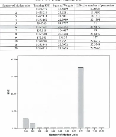
This section describes the experiments performed to determine the optimal number of hidden units to represent the model. For this purpose, the number of hidden units is varied fiom 1 to 20, and the model was evaluated each time the number of hidden units is changed. The MLP training was performed for 500 epochs (cycles) while the SSE performance function was used to evaluate the convergence of the MLP each time a hidden unit is added or removed. The optimal hidden layer size was found to be 6 for both 'defects' and 'time' models. The MLP training results for the 'defects' model is shown in Table 1 and Table 2.

Prosiding Seminar Kebangsaan Pengoptimuman Berangka dun Penyelidikan Operasi Ke-2

[image:5.595.104.495.265.729.2]

13-14 Disember 2008

Table 1: MLP structure results for 'defects'

Table 2: MLP structure results for 'time'

Effective number of parameters 8.40997

15.8015 24.0872 24.6359 25.9243

-" * '

y

;&.P;r?;3.

27.3663 27.1874 127.0000 27.0322 27.0754 27.1995 Number of hidden units

1 2 3 4 5 m.. " > <

" - > j - , ,-A

1.00 2.00 3.00 4.00 5.00 6.00 7.00 8.00 9.00 10.00 15.00

Number of Hidden Units

Figure 2: SSE comparison for 'defects' model Training SSE 5.617 2.92256 0.335414 0.347128 0.295796

*rc A/*" L

6 ;

b;;e:W*, ,, ,, A ,

Effective number of parameters 6.70823

11.5896 18.1518 23.1391

71

ij$;,?$& 4 ~ ; : *$;

:;9$p@@&$22

>;* > ' -99 21.6147 127 22.6917 22.3548 22.9966 Squared Weights 74.1111 22.1726 56.3065 43.4658 37.9359

;

* 3 \b<& $ 2 <

<$

.,

*.4:

Squared Weights 43.6819 25.628 1 21.5081 22.3989 84.1777

-""'"""'w '.~'-

&h

:&3~33$&3*K3;i

104.687 20.33 18 136.32 22.255 1 22.7972 2 1.7665 Number of hidden units

1 2 3 4 5

30.00

W

V)

V) 20.00

10.00

0.00

1.00 2.00 3.00 4.00 5.00 6.00 7.00 8.00 9.00 10.00 15.00 20.00

[image:6.595.131.475.77.354.2]

Number of Hidden Units

Figure 3: SSE comparison for 'time' model

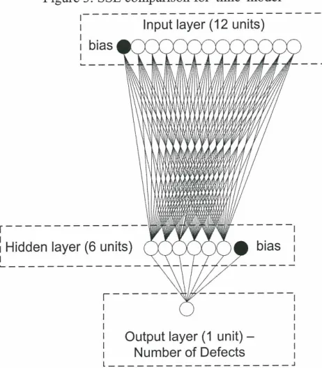
I--- I I Input layer ( I 2 units) ! I

I bias I

k - - -

[ - - -

I Hidden layer

(6 un

I

- - -

r---

I I

I I

1 Output layer ( I unit) - I I

I Number of Defects I I L - - - J

[image:6.595.184.415.376.640.2]

Prosiding Seminar Kebangsaan Pengoptimuman Berangka dun Penyelidikan Operasi Ke-2 13-1 4 Dkember 2008

I - - - - _ - - - _ - - _ _ - _ - - -

I

I

Input layer ( I 2 units)

I

i

bias

I L - - -

r - - -

I

I Hidden layer (6 units) I

- - -

r - - - - - -

I

I

I I

I Output layer (I unit) - I

I

I Manufacturing Time I I

[image:7.595.181.413.90.352.2]

L - - - _ - - - J

Figure 5: Optimal MLP structure for 'time' model

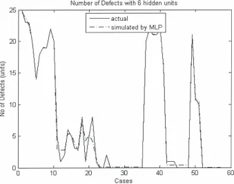
Number of D~fects with 6 hidden units 25

20 30 40 50

Cases

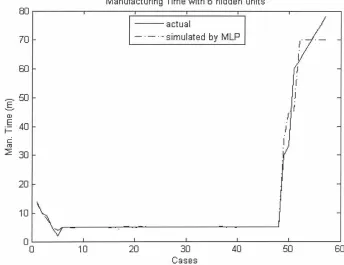
[image:7.595.126.465.392.658.2]

Manufacturing Time with 6 hiddsn units

0

Q 10 20 30 40 50 60

Cases

I 1 I I I

[image:8.595.121.465.83.348.2]

- . - . - _{simulated by MLP}

Figure 7: Modelling results for 'time' model (12 variables)

.

! 1 I

CONCLUSIONS

I

J -

i

-

Particle swarm optimization (PSO) has obvious ties with evolutionary computation. Conceptually, it seems to lie somewhere between genetic algorithms and evolutionary programming. It is highly dependent on stochastic processes, like evolutionary programming. The adjustment toward pbest and gbest by the article swarm optimizer is conceptually similar to the crossover operation utilized by genetic algorithms. It uses the concept of fitness, as do all evolutionary computation paradigms. Much further research remains to be conducted on this simple new concept and paradigm. The goal in developing it has been to keep it simple and robust, and we seem to have succeeded at that.

-

-

-

I I I I I

We also found that the selection of the optimisation algorithm has a significant effect on the suitability of the final model. For the two optimisation algorithms considered here, the particle swarm optimisation algorithm significantly outperformed the genetic algorithm. Also, the particle swarm optirnisation algorithm is much easier to configure than the genetic algorithm and is more likely to produce an acceptable model.

Future work will include investigation of the PSO's performance in other benchmark and real(1ife problems, as well as the development of specialized operators that will indirectly enforce feasibility of the particles and guide the swarm towards the optimum solution, as well as fine-tuning of the parameters that may result in better solutions.

REFERENCES

Milligan, G. W. and Cooper, M. C.. 1986. A study of the comparability of external criteria for hierarchical cluster analysis. Multi-variate Behavioral Research, 2 1,44 1-458.

Hartigan, J.A. (1975), Clustering Algorithms, New York: John Wiley & Sons, Inc.

Hartigan and Wong, 1978. Algorithm AS 136: a k-means clustering algorithm. Appl. Statist. v28. 100- 108.

Prosiding Seminar Kebangsaan Pengoptimuman Berangka dun Penyelidikan Operasi Ke-2 13-1 4 Disember 2008

Johnson, P. (1987).

SPC

for short runs: A programmed instruction workbook. Southfield, MI: Perry

Johnson.

Montgomery, D. C. (1991) Design and analysis of experiments (3rd ed.). New York: Wiley.