Exponential Dynamical Anderson Localization in
N-particle Models on Graphs with Infinite-range
Interaction
Victor Chulaevsky
Department of Mathematics, University of Reims Champagne-Ardenne, France
Copyright c⃝2015 by authors, all rights reserved. Authors agree that this article remains permanently open access under the terms of the Creative Commons Attribution License 4.0 International License
Abstract
We extend the techniques and results of the multi-particle variant of the Fractional Moment Method, developed by Aizenman and Warzel, to disordered quantum systems in general finite or countable graphs with polynomial growth of balls, in presence of an exponentially decaying interaction. In the strong disorder regime, we prove complete exponential multi-particle strong localization. Prior results, obtained with the help of the multi-scale analysis, proved only a sub-exponential decay of eigenfunction correlators.Keywords
Multi-particleAnderson Localization, Eigen-valueConcentrationEstimates1
Introduction
2
Introduction: The motivation and
the model
The rigorous multi-particle Anderson localization theory is a relatively recent direction in the spectral theory of dis-ordered media. The first results in this direction, establish-ing the stability of Anderson localization in a two-particle system in Zd with respect to a short-range interaction [16], have been immediately followed by the proofs of exponen-tial spectral localization (cf. [5, 17]) and exponenexponen-tial strong dynamical localization (cf. [5]) inN-particle systems, for any fixedN≥2.
In the multi-particle models with finite-range interaction, the MPFMM, when applicable, provides the strongest decay bounds upon the eigenfunction correlators (EFC), as does its original, single-particle variant. In particular, such bounds are stronger than those proved with the help of the multi-particle MSA (MPMSA), provided both methods apply to the same model. However, the relations between the two approaches are more complex in the realm of multi-particle, interactive models than for the systems with no interaction. In particular, in the situation where the interaction poten-tial decays slower than exponenpoten-tially, the existing techniques (based on the MPFMM or the MPMSA) allow one to prove
only a sub-exponential decay of the EFCs; in the case of the MPFMM this results in a similar – sub-exponential – decay of the eigenfunctions, for the latter is derived from the anal-ysis of the fractional moments and, ultimately, of the eigen-function correlators. The MPMSA is free from this limita-tion, since one can carry out independent analyses of the EFC and of the EFs. Exponential decay of the EFs in presence of a sub-exponentially decaying interaction was proved in dis-crete N-particle Anderson models (cf. [19]) and in a class of continuous models with the so-called alloy-type random potential (cf. [11]).
For these reasons, we consider in the present paper only the case of exponentially decaying interactions, where an ex-tension of the MPFMM techniques developed by Aizenman and Warzel [5] allows us to prove exponential decay of the eigenfunctions and of their correlators.
2.1
The multi-particle Hamiltonian
Consider a finite or countable connected graph(Z,E) with-out cyclic edges endowed with the canonical graph distance d = d(Z):d(x, y)is the length of the shortest path fromxtoy
over the graph edges;d(x, x) = 0. We assume that
∀L≥1 sup x∈Z
card BL(x)≤CdLd.
Further, consider the Cartesian powerZN,N ≥2, with the graph structure defined as follows: x = (x1, . . . , xN) and y = (y1, . . . , yN) form an edge iff there exists j such that d(xj, yj) = 1 and xi = yi for all i ∈ {1, . . . , N} \ {j}. The graph with the vertex setZN and the defined edge set will be denoted byZN. ForZ =Zd, this construction gives rise to the graph(Zd)N ∼=ZN dwith the usual graph structure.
The vertices ofZN represent the configurations ofN
dis-tinguishable quantum particles inZ. An important character-istics of x = (x1, . . . , xN)is its support Πx := {x1, . . . , xN}. (Notice that in a system of N indistinguishable Fermi-particles, Πxis the configuration.) We define the diameter of a configuration by
diamx≡diam Πx= max
It will be convenient to use also the max-distance inZN, ρ(x,y) = max
1≤i≤Nd(xi, yi), (2.2) and the so-called Hausdorff (pseudo-)-distance, defined ac-tually for the supportsΠx,Πyand formally extended to the configurations:
dH(x,y) = max
[
max
x∈Πxd(x,Πy),ymax∈Πyd(y,Πx)
]
. (2.3) A more natural object than the max-distance is its sym-metrized counterpart
dS(x,y) = min π∈SN
ρ(x, π(y)); (2.4) here the elementsπof the symmetric groupSN act on con-figurations by permutations of the particle positions. As we explain below, the localization bounds in our model can be established only in terms of a permutation-invariant metric in theN-particle configuration space. Note thatdH is also permutation-invariant. An important relation betweendSand
dHis the following inequality:
dH(x,y)≥dS(x,y)−min[diamx,diamy]. (2.5)
We study a random bounded self-adjoint operator in
ℓ2(ZN), of the form
H(ω) = N
∑
j=1
(
−∆(j)+gV(xj;ω)
)
+U(x),
whereV : Z ×Ω → R is a random field onZ (the single-particle configuration space), relative to some probability space(Ω,F,P),Uis the operator of multiplication by the func-tion
x= (x1, . . . , xN)7→
∑
i̸=j
U(|xi−xJ|),
generated by a two-body interaction potentialN∋r7→U(r), and∆(j)are replicas of the canonical graph Laplacian onZ, acting on the respective variables (particle positions)xj.
2.2
Assumptions
We assume that the interaction potential satisfies the fol-lowing condition.
(U1)∀r≥0 |U(r)| ≤Ce−ar, C, a∈(0,+∞).
Our main assumption on the external (random) potential is as follows.
(V1)The random fieldV :Z ×Ω→Ris IID, a.s. bounded, with
P{V(x;ω)∈[0,1]}= 1,
and admits a bounded marginal probability densitypV(·). The assumption of positivity is not essential, for a bounded random potentialV, since one can introduce a new potential
e
V(x;ω) := V(x;ω)−infV ≥ 0, and this simply results in a global energy shift, leaving invariant all eigenfunctions. Re-stricting the support to the interval [0,1] is convenient, but does not result in a loss of generality, due to the presence of the amplitudegin the random potentialgV(·;ω).
2.3
Main results
Theorem 2.1. Assume that the interaction potentialUin the Hamiltonian H(ω) decays exponentially fast at infinity (cf. Assumption(U2)) and the external random potential satis-fies Assumption(V1). Forg0large enough and for allgwith |g| ≥g0,H(ω)exhibits exponential decay of the fractional
mo-ments of the Green functions. Specifically, letI⊂Rbe an in-terval of length|I|<∞, then there exists somem=m(g)>0
such that for any pair ofN-particle configurationsx,yone
has ∫
RE
[
|G(x,y;E)|s]dE≤ |I|e−mdH(x,y). (2.6) Remark 2.1. m(g)→+∞as|g| →+∞.
Theorem 2.2. Consider anN-particle Anderson model with the single-particle configuration spaceZ1 and the
Hamilto-nian
Hh(ω) =−∆+gV(x;ω) +hU(x), h∈R.
Assume that the inter-particle interaction potentialUdecays exponentially fast at infinity (cf. Assumption(U2)) and the external random potential satisfies Assumption(V1). For any
g ̸= 0there existm >0 andh◦ =h◦(|g|, FV,∥U∥) >0 such
that for all h ∈ [−h◦, h◦], the random Hamiltonian Hh(ω)
exhibits exponential decay of the fractional moments of the Green functions: for any bounded intervalI⊂R,
∫
IE
[
|G(x,y;E)|s]dE≤ |I|e−mdH(x,y). (2.7)
Theorem 2.3. The exponential decay of the fractional mo-ments of the form (2.6)–(2.7)implies complete exponential strong dynamical localization: for any configurationsx,y
E
[
sup t∈R⟨
1y|e−itH(ω)|1x
]
≤C(x)e−m′dS(x,y). (2.8)
Our proofs are closer to the original technique from [5] than to a more advanced method developed by Fauser and Warzel [21].
3
Basic notation and preliminary
re-marks
We will systematically make use of the elementary in-equality which is one of the cornerstones of the FMM tech-nique:∀s∈(0,1)∑nans≤∑n|an|s.
Another standard ingredient of the localization analysis is the second resolvent identity,(A+B)−1=A−1−A−1B(A+
B)−1=A−1−(A+B)−1BA−1, valid as long asAand(A+B) are invertible elements of some algebra. It will be always used in a situation where A andB are linear operators in finite-dimensional (Hilbert) spaces, so there is no need to ad-dress the issue of boundedness and domains. Often, albeit not always, it will be used in the case whereA=A1⊕A2:H → H, H=ℓ2(Λ1)⊕ℓ2(Λ2)∼=ℓ2(Λ1⊔Λ2), Aj:ℓ2(Λj)→ℓ2(Λj),
Λj ⊂ Zbeing finite subsets with the boundariesDj=∂−Λj, D1∩ D2=:D ̸=∅. As to the operatorB, it has the form (in Dirac’s ”ket-bra” notation)
∑
⟨xy⟩
(
where ⟨xy⟩ runs over all pairs with x ∈ D1, y ∈ D2 and d(x, y) = 1. In this case the resolvent equation takes the form often called the Geometric Resolvent Equation (GRE) and implies the Geometric Resolvent Inequality (GRI), some-times also referred to as the Simon–Lieb Inequality (SLI). Its FMM-flavoured variant (which will be referred to as the FGRI = Fractional GRI) reads as follows:
|GΛ(x, y;E)|s≤
∑
⟨w,w′⟩∈D1×D2
|GΛ1(x, w;E)|
s|G
Λ(w′, y;E)|s.
Following [5], we introduce the energy-disorder expecta-tion bEI[·]: given an interval I ⊂ Rof length|I| ≥ 1and a measurable functionf:R×Ω, we set
b
EI[f(E, ω) ] :=|I|−1∫ IE
[f(E, ω) ]dE,
whereE[·]is the conventional expectation relative to(Ω,P). The benefits of averaging over the augmented, energy-disorder probability space are two-fold:
1. In the fractional moment analysis of the Green func-tions, it allows one to focus on the decay properties of the eigenfunction correlators and prove a crucial result on finiteness of the fractional moments by a “soft” argu-ment, based on the Boole identity (cf. Appendix C) and an explicit integration in the energy.
2. The derivation of the decay bounds on the eigenfunc-tion correlators from the bounds on the fraceigenfunc-tional mo-ments of the Green functions, used in our paper (cf. Sect 3.1), employs a Chebyshev-type argument in the energy-disorder space rather than in the disorder space, so the bounds in terms of the expectationsEbI[·]turn out to be a natural tool for such a derivation.
The following elementary statement explains what makes the2-particle systems special in the framework of our analy-sis:
∀x,y∈ Z2 dH(x,y) = dS(x,y).
For example, withZ=Zd, the Hausdorff distance is the sym-metrized version of the genuine norm-distance in (Zd)2 ∼=
Z2d. Thus the2-particle decay estimates established in the Hausdorff distance imply those in the (symmetrized) norm-distance.
3.1
Finiteness of the fractional moments
A priori bounds on the fractional moments of the resol-vents have been one of the inescapable ingredients of the FMM since its inception in [1]. Their adaptation to the multi-particle models (cf. [5]) is, however, more involved than in the1-particle theory. Both Ref. [5] and a more recent work [21], as well as [4] dedicated to the FMM for differential ran-dom operators, refer to some general results on maximally dissipative operators and related topics; cf., e.g., [4], [8, 33].We will need the following statement.
Lemma 3.1. For any s ∈ (0,1) there exists Cs < ∞ such that for any finite connected subset Λ ⊂ Z, any two sites
u1, u2 ∈ Z, withn:= card{u1, u2} ∈ {1,2}, and any pair of
configurationsx,y∈Λ2withΠx∋u1,Πy∋u2, the following
bound holds:
E[|G(x,y;E)|sF̸=u1,u2
]
≤Ms<+∞, (3.1)
where
Ms=Ms(s, g, FV, n)≤C(FV, n)|g|−s, (3.2)
for someC(FV, n)<∞.
In Ref. [5], the proof of such an a priori bound has been clearly outlined, with direct references to prior works con-taining necessary analytic and probabilistic results and mak-ing the proof complete; it does not rely on any specific form of the interaction potential, be it of finite or infinite range, since only the random potential is used in the main argu-ment. However, for the reader’s convenience, we provide in Appendix D a detailed, self-contained proof of Lemma 3.1 relying on a bare minimum of analytic tools, including the Birman–Schwinger relation for finite-dimensional operators and the Boole formula [7] (proved in Appendix C; the re-markably short and elementary argument is due to Loomis [28]). The proof shows thatMsis a continuous function of the interaction potential. In particular, for the interaction of the formhU(x), with fixedU(·)andh∈R, it depends continu-ously onh; this fact is used in the application of the MPFMM to the perturbations of the non-interactingN-particle system by weak interactionshU,|h| ≪1.
3.2
From the fractional moments to the EFCs
This subsection may prove to be of limited interest to a reader familiar with modern methods of derivation of strong dynamical localization from the suitable estimates, in prob-ability or in expectation, obtained through a fixed-energy lo-calization analysis. The main goal here is to show that the scaling analysis performed in Section 3 implies indeed N -particle dynamical localization for any givenN >1, provided the localization for the single-particle systems is sufficiently strong.We employ an argument developed by Elgart et al. [20]; this is in essence an advanced version of an older Chebyshev-type argument given by Martinelli and Scoppola [29] in the general context of the MSA (the FMM was not known yet in 1985). Its form given below appeared in [9] and [18].
Given a ballBL(z), introduce a function (E, ω)7→Fz(E;ω)≡Fz,L(E;ω)
:= max
y∈∂−BL(z)
|GBL(z)(z,y;E;ω)|.
In a number of formulae below, the radius Lwill be fixed (and clear from the context), so it will be often omitted from notationFz,Lfor brevity.
We denote by Σ(HBL(z)(ω))the (finite) spectrum of the operatorHBL(z)(ω).
Lemma 3.2. Let be given a ballBL(z), a bounded interval
I⊂R, and real numbersaL, bL, cL, qL>0satisfying
bL≤min{aLc2L, cL} (3.3)
and
P{Fz(E;ω)> aL} ≤qL. (3.4)
Then there exists an eventSb,zsuch that P
{
Sb,z
}
≤b−L1qL
and for anyω̸∈ Sb,z, the set of energies
{E∈I:Fz(E;ω)>2aL}
is covered by a union of intervals
K∪z
i=1
centered at the eigenvaluesλj∈Σ(HBL(z)(ω))∩I.
Proof. Consider the random Borel subsets of I parameter-ized bya′>0(recall thatFzis continuous outside the finite
spectrum ofHBL(z))
Ea′,z(ω) ={E∈I:Fz(E)> a′}
and, withaLsatisfying (3.3), the events parameterized byb′> 0:
Sb′,z:={ω: mes (EaL,z)> b′}.
Assuming (3.3)–(3.4), apply Chebyshev’s inequality and the Fubini theorem:
P{SbL,z
}
≤b−L1E
[ ∫
I
1Fz(E)>aLdE
]
=b−L1
∫
IE
[
1F z(E)>aL
]
dE
=b−L1
∫
IP{
Fz(E)> aL}dE≤b−L1|I|qL. (3.5)
Fix anyω̸∈ SbL,z, so thatmes (Ez(aL;ω))≤bL, and consider the random sets parameterized byc′>0:
R(c′) :={λ∈R: min
j |λj(ω)−λ| ≥c
′}.
Note that for0< bL≤cL, we have
AbL:={E: dist(E,R(2cL))< bL} ⊂R(cL),
hence the setAc
bLis a union of sub-intervals at distance≥cL from the spectrum. Let us show that
∀ω̸∈ SbL,z {E:Fz(E;ω)≥2aL} ∩R(2cL) =∅.
Assume otherwise and pick any point λ∗ in the non-empty intersection figuring in the LHS. LetJ := {E′ : |E′−λ∗|< bL} ⊂AbL⊂R(cL), so for anyE∈Jwe have∥G(E)∥ ≤c−L1. Further, by the second resolvent identity, for anyE ∈ J we have
∥G(E)∥ ≥ ∥G(λ∗)∥ − |λ∗−E| ∥G(λ∗)∥ ∥G(E)∥
≥2aL−bc−L2≥aL,
owing to (3.3). Therefore,Eb⊃J, which is impossible, since mesEbL,z(ω)≤bLwhilemesJ= 2bL.
The obtained contradiction completes the proof.
Theorem 3.1. Let be given a bounded intervalI ⊂ Rand real numbersaL,bL,cL,qL>0satisfying(3.3)and
max
z∈{x,y}Esup∈IP{
Fz(E)> aL} ≤qL. (3.6)
Assume also that for some functionf: [0,1]→R+one has
P{dist(Σ(HBL(x)),Σ(HBL(y))
)
≤s
}
≤f(s). (3.7)
Then
P{ ∃E∈R: min{Fx(E),Fy(E)}> aL} ≤2|I|b−1qL+f(4cL).
(3.8)
Proof. Introduce the events SbL,z =
{
ω : mes{E ∈ I :
Fz(E)> aL} > bL
}
, and the random setsEaL,z(ω) :={E ∈
I : Fz(E;ω) > aL}, for z ∈ {x,y}, as in Lemma 3.2. By Lemma 3.2, we haveP{SbL,z
}
≤b−L1|I|qL, so for the event SbL := SbL,x∪ SbL,y one has P
{
SbL
}
≤ 2b−L1|I|. For any
ω̸∈ SbL, each of the two setsEaL,x(ω),EaL,y(ω)has Lebesgue measure bounded bybL, thus
P
{
sup E∈I
min
z∈{x,y}Fz(E)> aL
}
≤P{Ex,aL∩Ey,aL̸=∅}
≤P{ S }+P{ {Ex,aL∩Ey,aL̸=∅
}
\ SbL
}
≤2b−L1|I|+P{ {Ex,aL∩Ey,aL̸=∅}\ SbL
}
.
By construction of the setEz,aL,z∈ {x,y}, for anyω̸∈ SbL it is contained in the2cL-neighborhood of the spectrumΣz(ω)
ofHB
L(z)(ω), hence
P{ {Ex,aL∩Ey,aL̸=∅
}
\ SbL
}
≤P{dist(Σx(ω),Σy(ω))≤4cL
}
≤f(4cL),
by virtue of the eigenvalue comparison bound (3.7). This completes the proof.
It is readily seen that the condition (3.3) is fulfilled with
aL= e−
1
3mL, bL= e−23mL, cL= e−18mL, qL= e−mL,
The proof of the above theorem relies on the EV compari-son bound (3.7). For our purposes, it would suffice to quote Ref. [15] where a suitable bound was proved.
Note also that in the context of multi-particle Ander-son models in a continuous configuration space (Rd), Klein and Nguyen [27] recently improved and extended the multi-particle two-volume bound to a large class of alloy-type An-derson Hamiltonians; in particular, this class is larger than the one considered in Refs. [12, 21].
Proposition 3.2 (Cf. [26]*Corollary 2.4). Assume that the marginal probability distribution of the random potentialV
admits a bounded densitypV. Then for any pair ofN-particle
configurationsx,ywithdH(x,y)>2L, one has
P{dist(Σ(HBL(x)),Σ(HBL(y)))≤ϵ} ≤C(N)L2N d∥pV∥∞ϵ.
(3.9)
The next statement is given in the form presented in [9] and [18], but the credit goes essentially to Germinet and Klein [22] who proved a stronger and more general result. It refers to an intervalI⊂R, to be consistent with the previous discus-sion. However, unlike Theorem 3.1 where integration overI
is performed, here the boundedness ofIis not important; for example, one could takeI =R, provided the validity of the hypothesis (3.10) is established inI=R.
Theorem 3.3(Cf. [9]*Lemma 9). Given a positive integer
L, assume that the following bound holds true for a pair of disjoint ballsBL(x),BL(y)and someaL, hL>0:
P
{
sup E∈I
min[Fx(E),Fy(E)]> aL
}
≤hL. (3.10)
Then for any finite connected graphG⊃BL(x)∪BL(y)one
has
E
[
sup ϕ∈B1(R)
⟨1x|ϕ(HΛ)|1y⟩
]
≤2aL+hL. (3.11)
Proof. Fix a finite graphG ⊃ BL(x)∪BL(y). The random operatorHG(·)has a finite orthonormal basis{Ψi(·)}with as-sociated EVs{Ei(·)}. Let
SL=
{
ω: sup E∈I
min[Fx(E),Fy(E)]> aL
}
By hypothesis,P{ SL} ≤ hL. Fix someω ∈ SLc = Ω\ SL and suppose that for each eigenvalue Ei = Ei(ω) there is zi∈ {x,y}such thatBL(ziisEi-NS; let{vi}={x,y} \ {zi}. DenoteYx,y:=⟨1x|ϕ(HΛ)|1y⟩, then by the GRI for the ball
BL(zi)we have, withωfixed and omitted from notation for brevity,
Yx,y≤ ∥ϕ∥∞
∑
Ei∈I
Ψi(x)Ψi(y≤
∑
Ei∈I
Ψi(vi)Ψi(zi)
≤ ∑
Ei∈I
Ψi(vi)hL(CLN d)−1
∑
(u,u′)∈∂−
Ψi(u)
≤ hL
CLN d
∑
Ei∈I
Ψi(u)
∑
(u,u′)∈∂−
(Ψi(x)+Ψi(y))
≤ hL|B|
CLN dmaxu∈G 1 2
∑
Ei∈I
(2Ψi(u)2+Ψi(u)+Ψi(u))
≤hL 2 umax∈G
(
21u2+1x2+1y2)≤2aL, where the last line follows from Bessel’s inequality. Hence
E[Yx,y]≤E
[
1Sc
LYx,y
]
+E[1SLYx,y]≤2aL+hL.
Collecting Theorems 3.1 and 3.3 and Proposition 3.2, we come to the following conclusion.
Theorem 3.4. Suppose that the following condition is ful-filled: for someR0∈Nand allN∋R≥R0, for any
configu-rationsx,y∈ZN withdH(x,y)>2R
max
z∈{x,y} Esup∈IP
{
Fz(E)>e−13mR
}
≤e−mR. (3.12)
Then for any pair of configurations x,y ∈ ZN with
dH(x,y) > 2R ≥ 2R0 and finite connected subgraph G ⊃ BR(x)∪BR(y)one has
E
[
sup ϕ∈B1(R)
⟨1x|ϕ(HG)|1y⟩
]
≤(C1|I|+C2) e− 1
3mR+C3e− δ
8mR.
(3.13)
Furthermore, on account of the geometrical inequality
dH(x,y)≥dS(x,y)−diam Πx= dS(x,y)−C(x),
one has, therefore,
E
[
sup ϕ∈B1(R)
⟨1x|ϕ(HG)|1y⟩
]
≤Const(x)e−µdS(x,y). The dependence of the RHS factor onx, throughdiam Πx, renders the dynamical localization bound non-uniform in the
N-particle configuration space, for N ≥3, while forN = 2 one can actually replace Const(x) by an absolute constant, owing to the equivalence betweendSanddHin this particular
case.
3.3
From EFCs to GFs
In this subsection we provide a detailed proof of a fairly general relation between the resolvents and the EF correla-tors, which had been used in numerous works on the FMM. The single- or multi-particle nature of the Hamiltonian at hand is irrelevant, as long as the fractional moments of the EFC can be effectively assessed in the intended application(s) of the general relation. Recall that it suffices for our purposes
to establish strong dynamical localization in arbitrarily large but finite domains in the configuration space (with the re-maining work to be done with the help of the Fatou lemma, as in [2, 3, 4]), so we can indeed restrict our analysis to the finite-dimensional operators.
Lemma 3.3. Let H = HG be an N-particle Hamiltonian in a finite graph G, and G(x,y;E) the kernel of its resol-ventG(E) =(HΛ−E
)−1
andQ(x,y)the EF correlators (we choose the eigenfunctions real)
Q(x,y) =∑ i
ψi(x)ψi(y).
Then for any bounded intervalI⊂Rand anys∈(0,1)
∫
I|
G(x,y;E)|sdE≤ 2|I| 1−s
1−s (Q(x,y))
s. (3.14)
Proof. In this deterministic statement, the EFs are fixed, and the only relevant variable isE. Fix the pointsxandy. The GF is a rational function, and we divide it into the sum of two terms, according to the signs of the numerators:
G(x,y;E) = ∑ Ei:ci≥0
ci
Ei−E
+ ∑
Ei:ci<0
ci
Ei−E
=:G+x,y;E) +G−x,y;E).
We have
∫
I|
G(E)|sdE≤
∫
I|
G+(E)|sdE+
∫
I|
G−(E)|sdE
Both integrals are assessed in the same way, so we focus on the first one.
It is convenient at this point to introduce probabilistic lan-guage, as we are going to apply a standard technique for the probability distribution functions (PDF), and consider the probability space(I,BI,mesI), whereBIis the Borel sigma-algebra andmesI :=|I|−1mes the normalized (i.e., probabil-ity) Lebesgue measure inI⊂R. Further, consider the mea-surable functionG±:E7→G±(E)(i.e., a ”random variable” on(I,mesI)), and letF±(t)be the PDF of its absolute value:
F±(t) = mesI{E:|G±x,y;E)| ≤t}. Then
∫
I|
G±(x,y;E)|sdE=|I|bEI[|G±(x,y;E)|s] =|I|
∫ ∞
0
tsdF±(t).
Using integration by parts for the Stiltjes integral, we obtain for anys >0
∫ ∞
0
tsdF±(t) =s
∫∞
0
ts−1(1−F±(t))dt,
where both integrals converge or diverge simultaneously. The goal of this transformation is to reduce the estimate to that of the tail distribution function t 7→ 1−F±(t) = mesI{E : G±(E)> t}, with the help of the Boole identity (cf. Proposi-tion C.1), applicable to any raProposi-tional funcProposi-tion with simple, real poles and positive expansion coefficients,f:t7→∑ni=1 ci
ti−t, and stating that
mes{λ: |f(λ)|> t}=2
∑n i=1ci
hence
mesI{λ:|f(λ)|> t} ≤
2∑ni=1ci |I|t ,
Recall that, in fact,ci=ψi(x)ψi(y)(we choose the EFs real), so that
∑
i:ci≥0
ci≤Q+(x,y),
∑
i:ci<0
(−ci)≤Q−(x,y), whereQ±(x,y)are components of the EF correlator:
Q+(x,y) +Q−(x,y) = ∑ i:Ei∈I
|ci| ≤Q(x,y).
Thus, denoting for brevityQ±≡Q±(x,y), we have 1−F±(t)≤min
(
1,2Q±(|I|t)−1
)
=1[0,2Q±/|I|](t) +2Q±
|I|t 1[2Q±/|I|,+∞)(t)
and
∫∞
0
tsdF±(t)≤s
∫ ∞
0
ts−1(1−F±(t))dt. ≤s
∫ 2Q/|I| 0
ts−1dt+ 2sQ±
∫∞
2Q/|I|
ts−2dt
=
(2Q
±
|I|
)s
+ 2sQ±(2Q±) s−1 |I|s(1−s)
=(2Q±) s|I|−s 1−s .
Therefore, usingαs+2βs ≤(α+β 2
)s
, s <1, we obtain
∫
I|
G(x,y;E)|sdE≤ |I| ·2
s|I|−s
1−s (Q+(x,y))
s+Q
−(x,y))s)
≤2(Q(x,y))s|I|1−s
1−s .
4
Decay of the fractional moments of
the GFs
Following [5], we will use the sequence of length scales
{Lk, k≥0}defined by
Lk+1:= 2(Lk+ 1), k= 0,1, . . . , (4.1) or, explicitly,
Lk= 2k(L0+ 2)−2. (4.2)
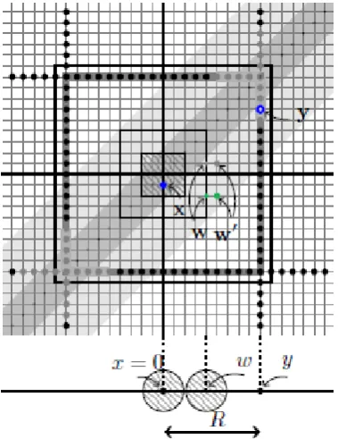
We consider two N-particle configurations x,y with R := dH(x,y) ∈ (Lk, Lk+1] for some k ∈ N, and choose some a∈ Πx,y ∈ Πy such thatR= d(a, y). Such pointsa, y ex-ist by definition of the Hausdorff dex-istance.
On Fig. 1, where the caseZ = Z1 is illustrated, we set
a= 0, by translation invariance of the random potential in the 1-particle configuration space.
Introduce the following notation:
XΛ L(u) =X
Λ,N
L (u) ={x∈Λ
N : Πx∋u,diam Πx≤L}. (4.3) Equivalently, settingu= (u, u, . . . , u),XΛ
L(u) = ΛL(u)∩ΛN is the set of allN-particle configurations in the ”physical” domainΛat distance≤Lfrom the positionu.
For notational brevity, the Green functionsG(x,y)with no subscript (and the energyEusually omitted from notation, as
we perform afixed-energyanalysis in the scaling procedure) refer to the Hamiltonian in the above mentioned large – and fixed – domainΛ.
In order to successfully carry out the scale induction, one needs of course some technical assumptions relative to the fractional moments and eigenfunction correlators at a (prop-erly chosen) initial scaleL0. Such initial scale estimates will
appear in the course of the induction step; their validity at the scaleL0is discussed in Section 5 below.
As to the magnitude ofL0suitable for the induction, it can
be arbitrary for the proof of localization at large disorder: the largerL0, the larger must be the amplitude|g|of the random
potential guaranteeing the onset of the N-particle localiza-tion. The strong disorder manifests itself in a very clear way – through a small constantMs≤C|g|−sfiguring in a number of formulae.
However, in the case of an N-particle system in one di-mension, with possibly small disorder amplitude |g|, one has to chooseL0 large enough, to ensure that the decay of
GFs/EFs/EFCs at distanceL0is perceptible. See a brief
dis-cussion of the Lyapunov exponents in one dimension in Sec-tion 5.2.
Assumption for the stepN−1 N,N≥2.
For alln∈[1, N−1], the EF correlatorsQ(n)(x,y)ofn-particle systems in the domainΛfulfill the following condition: for someA, mN−1>0and allx,y∈XΛL,n
E[Q(n)(x,y)]≤Ae−mN−1dH(x,y). (4.4)
Observe that the expectation in (4.4) is relative only to the disorder, since the EFCs do not depend upon energy.
The rest of this section is the central part of the paper. Its role and relations with other sections can be described as fol-lows.
1. Below we focus on the derivation of exponential decay bounds on the fractional moments of theN-particle sys-tem inΛ, with somemN ∈ (0, mN−1)to be chosen
ap-propriately.
2. The validity of the assumption (4.4) forN = 2, i.e., rel-ative to the 1-particle systems, is discussed in Section 5. It follows from the well-known results of the single-particle fractional moment analysis.
3. Once the exponential decay bounds on the fractional moments of theN-particle GFs are established, the cor-responding exponential bounds on theN-particle EFCs (required for the next step of the induction on the num-ber of particles, N N + 1) will follow from the general arguments given in Sect. 3.2. An important (and unfortunate) feature of the existing methods of the multi-particle Anderson localization theory, including the MPFMM, is a deterioration of the decay ratemnat each induction stepn n+ 1:
m1> m2· · ·> mN−1> mN. (4.5) In fact, both the MPMSA and the MPFMM result inmN ∼
O(m1/(N−1)!).
For notational brevity, below we often drop the subscripts from the notations for the decay rates likemn. We work here with theN-particle systems and their subsystems ofn≤N−1 particles inΛ, so the minimal decay rate is given bymN−1>
Theorem 4.1. FixN ≥2and assume that for alln= 1, . . .,
N−1, the exponential decay of theEFCs is established, in the Hausdorff distance(s) for n-particle Hamiltonians H(n)(ω)
with decay exponentsm1> m2>· · ·> mn−1. Then for some c >0, theN-particle HamiltonianH(N)(ω)also feature ex-ponential decay of the EFCs in the Hausdorff distance, with decay exponentmN ≥cmN−1/(N−1).
Proof. The argument given below relies on Theorem 4.2. The case wheremax[diamx,diamy]> Lk/2can be analyzed separately, and we do so in Section 6. By Lemma 6.1, the assumptiondiamx> Lk/2along with (4.1) and the inductive hypothesis (4.4) imply
EI
[
|G(x,y)|s]≤Ae−cNmLk=Ae− cmN−1
N−1 Lk, c >0. (4.6)
Hence we can focus on the pairs of configurations of diameter
≤Lk/2.
SinceΠx∋aanddiamx≤Lk/2, we havex∈ BLk/2(a), where we denotea= (a, a, . . . , a). By construction,
min
[image:7.595.84.274.313.559.2]i d(xi, y) = d(Πx, y) = dH(x,y) =R > Lk, (4.7)
Figure 1.An example for the proof of Theorem 4.1. Hered= 1,N= 2.
thus y ̸∈ ΠBLk/2(a). By the FGRI applied to the cube
BLk/2(a),
b
EI[|G(x,y)|s]≤∂B
Lk/2(a)·
max
(w,w′)∈∂BLk/2(a)
b
EI[|G
BLk/2(a)(x,w)|
s|G(w′,y)|s] . (4.8) Here Πw′ = {w′, w′2, . . . , wN′ −1} with d(0, w′) = 12Lk + 1. Set u1 = w′, u2 = y. Then u1, u2 ̸∈ ΛLk/2(0), so GBLk/2(a)(x,w)isF̸=u1,u2-measurable, withF̸=u1,u2
gener-ated by{V(z;·), z∈Ω\ {u1, u2}}, so for any fixed pairw,w′
as above,
b
EI[|G
BLk/2(a)(x,w)|
s|G(w′,y)|s] ≤bEI[|G
BLk/2(x)(x,w)|sEbI
[
|G(w′,y)|sFΩ\{u1,u2}
] ]
.
(4.9)
Applying Lemma 3.1 (cf. Eqn. (3.1)), we obtain a uniform upper bound
b
EI[|G(w′,y)|sF
Ω\{u1,u2}
]
≤Cs|g|−s, (4.10) thus
b
EI[|G(x,y)|s]
≤Cs|g|−s∂BLk/2(a) bEI[|GB
Lk/2(x)(x,w)|
s]. Aplying the bound (4.13), we conclude that
b
EI[|G(x,y)|s]≤C
s|g|−s∂BLk/2(a) e
−cmLk.
Assessing the RHS expectation in (4.9) is the most tedious task, and it is entrusted to the multi-scale induction in Theo-rem 4.2. Introduce the following notations, to be used below withL=Lj+1) (cf. (4.3):
Υ(L) :=|∂BL(a)| sup Λ⊆BL(a)
∑
d(a,u)=L
x∈XΛL/2(a)
w∈XΛL/2(w)
b
EI[|G
Ω(x,w)|s].
(4.11) We also need a slightly modified quantity, defined for L=
Lj+1,j≥0:
e
Υ(Lj+1) :=|∂BLj+1(a)| sup Λ⊆BLj+1
∑
d(a,u)=Lj+1
x∈XΛ
Lj /2(a)
w∈XΛ
Lj /2(w)
b
EI[|G
Λ(x,w)|s].
(4.12) The correlatorsΥ(Lj),Υ(Lj+1)are required to carry out the
scale induction, butΥ(e Lj+1)are simpler to assess. Theorem 4.2. For allk≥0,
Υ(Lk)≤e−cmLk. (4.13)
Proof. Unlike Theorem 4.1, we consider now the pairsx,y
with Πx ∋ a, Πw ∋ w with specific values of the distance d(a, w) =Lj,j≥1, so the scale induction will be carried out only for such distances. To avoid confusion with the previ-ously used notation and arguments, the scales will be labeled by the indexj.
We havex∈BL
j/2(a)⊂BLj(a),w∈∂−BLj(a). Herew isLj/2-split and distant fromx: diamw> Lj/2,dS(x,w)≤ Lj/2, thus by Lemma 6.1,
b
EI[|G
BL(a)(x,w)|
s]≤Const e−cmLj
From this point on, we consider the configurationswof re-stricted diameter.
We aim to show first that the quantitiesΥ(Lj),j≥0, satisfy the recursion
Υ(2(Lj+ 1))≤
A′ |g|sΥ
2(L
j)+AL2jq+1e−
2νLj, (4.14) and then infer from (4.14) thatΥ(Lj)decay exponentially. Approximation by truncated correlators.Let us show that (cf. (4.11)–(4.12))
0≤Υ(Lj+1)−Υ(e Lj+1)≤2A·(Lj+1)2e−cmLj. (4.15)
Consider any term bEI[|G
Λ(x,w)|s]figuring in the sum for
Υ(Lj+1)but absent inΥ(e Lj+1). Its exclusion fromΥ(e Lj+1)
implies that 1
here the RHS inequality is due to the constraint figuring in the definition ofΥ(Lj+1). Both bounds ondiamware important.
First,Πx∋ aandΠw∋wwithd(a, w) =Lj+1, so it follows
from the upper bounddiamx≤Lj+1/2that
dH(x,w)≥d(a, u)−1 2Lj+1=
1 2Lj+1.
Next, the lower bounddiamw > Lj/2 enables us to apply Lemma 6.1 onR-distant configurations at least one of which isR-split; here we haveR= Lj/2withLj = 12Lj+1−1 ≥
1
3Lj+1, thus
b
EI[|G
Λ(x,w)|s]≤Ae−cmLj =Ae− c
3mLj+1,
so it remains only to assess the number of relevant terms. There are at mostCL2(j+1N−1)d choices for the pair (x,w), sinceΠw ∋ u withu fixed, Πx ∋ a, and diamx, diamw ≤
1
2Lj+1. Thus the number of terms which constitute the
dif-ferenceΥ(Lj+1)−Υ(e Lj+1)is bounded byCL2(j+1N−1)d. This
completes the proof of (4.15).
Recursion with truncated correlators. Consider the corre-latorΥ(e Lj+1). Introduce the configurationwb = (w, w, . . . , w)
(it plays the role similar to that ofa = (a, a, . . . , a), and de-note for brevityB′ =BLj(a),B′′ =BLj(wb),Λ′ = BL
j/2(0), Λ′′= BL
j/2(u). By the FGRI, we can write
b
EI[|G(x,w)|s]≤
∑
⟨z,z′⟩∈∂BLj(a)
⟨v,v′⟩∈∂BLj(w)
E[|GB′(x,z)|s|GB′′(v,w)|s·
·bEI[|G(z′,v′)|sF Λ′∪Λ′′
] ]
aiming, of course, to obtain a uniform upper bound on the conditional expectation in the RHS. To this end, notice that d(z′,a) = 1 +Lj/2, thusΠz′ ∋ z′ withz′ ̸∈ Λ′. Similarly, Πv′∋v′withv′̸∈Λ′′.
Therefore, the sigma-sub-algebraF̸=z′,v′generated by the random potential inZ \ {z′, v′}is larger thanFΛ′∪Λ′′, and
ap-plying Lemma 3.1 to the expectationEbI[·F
̸
=z′,v′
]
, we ob-tain
b
EI[|G(z′,v′)|sF Λ′∪Λ′′]
=EI[EI[|G(z′,v′)|sF̸=z′,v′] FΛ′∪Λ′′
]
≤ C gs.
Thus
b
EI[|G(x,w)|s] ≤ C
gs
∑
⟨z,z′⟩∈∂BLj(a)
⟨v,v′⟩∈∂BLj(w)
b
EI[|G
B′(x,u)|s]bEI[|GB′′(v,w)|s] .
Now considerbEI[|G
B′(x,u)|s]; the remaining expectation
in the RHS is assessed similarly. This is done in two steps: 1. Forzwithdiamu≤Lj/2we use the scale induction:
∑
⟨z,z′⟩∈∂BLj(a) diamu≤Lj/2
b
EI[|G
Λ′(x,z)|s]≤Υ(Lj).
2. Ifdiamz> Lj/2, then we apply Lemma 6.1:
b
EI[|G
Λ′(x,z)|s]≤Ae−m2Lj.
Collecting all possible verticeszof the categories (1) and (2), and upper-bounding the number of vertices from each category by|∂−Λ(x)|, we obtain
∑
z
b
EI[|G
Λ′(x,z)|s]≤C
(
Υ(Lj) +C′Lqje− mLj),
withq= 2(N−1)d. Similarly,
∑
v
b
EI[|G
Λ′′(v,w)|s]≤C|g|−s
(
Υ(Lj) +C′Lqje− m
2Lj).
DenoteMs= 2C|g|−s, then
e
Υ(Lj+1)≤
1 2Ms
(
Υ(Lj) +C′Lqje− m
2Lj
)2 .
where
Applying the approximation formula (4.15), we obtain Υ(Lj+1)≤
1 2Ms
(
Υ(Lj) +C′e− m
2Lj
)2
+ALpj+1e−m2Lj ≤ 1
2Ms
(
Υ(Lj) + e− m
3Lj
)2
+1 2e
−m
3Lj,
(4.16) providedL0is large enough (depending onm >0).
LetΥbj= Υ(Lj) + e− m
3Lj, then (4.16) can be re-written as follows:
b
Υj+1≤
1 2MsΥb
2 j+
1 2e
−m
4Lj. (4.17) In order to complete the induction step, we have to assume that
Ms1/2Υb0<1, (4.18)
thus
∃ν >0 : β0:= e2νM 1/2
s Υb0≤e−νL0. (4.19)
The validity of the assumption (4.18) (hence, that of (4.19)) is established in Section 5: (i) for strongly disordered systems, and (ii) for sufficiently weak perturbations of localized non-interacting systems in one dimension.
Denoteβk= e2νM 1/2
s Υbk,k≥0, then we have the recursion
βk+1≤
1 2e
−2νβ2 k+
1 2e
2νM1/2 s e−
m
4Lk
≤1
2e
−2νβ2 k+
1 2e
−m
5Lk,
(4.20)
provided thatL0 is large enough. A simple calculation (cf.
Lemma A.1) shows that (4.20) implies
with someµe≥cm >0(specified in Lemma A.1). This com-pletes Step 4 and the proof of exponential decay of the frac-tional moments of theN-particle Green functions. As was ex-plained before, the output from the induction stepN−1 N
for the GFs implies exponential decay of theN-particle EFCs (cf. Sect. 3.2). This makes possible the next induction step
N N+ 1, but only if the initial decay ratem1(cf. (4.5)) is
large enough, or, more to the point, if the obtained decay rate
mN for theN-particle systems is not too small – this is why the induction inNcannot be continued indefinitely.
5
Initial scale estimates for the
N
-parictle system
5.1
Strongly disordered systems in any
dimen-sion
The bounds for1-particles Hamiltonians, sufficient for our purposes, are established in a number of papers on the con-ventional Fractional Moment Method; cf. [1, 2, 3]. The scaling procedure in Section 4 allows one to establish the exponential decay bounds on the fractional moments of the
N-particle Green functions. Section 3.2 provides then the derivation of the exponential decay bounds on theN-particle eigenfunction correlators, thus completing the logical cycle
EF C(N−1) → GF(N) →EF C(N), i.e., the induction step
N−1 Nfor the EFCs.
5.2
Weakly disordered one-dimensional
sys-tems
Apart from the strongly disordered Anderson models in any dimension, Aizenman and Warzel [5] considered also the situation where the non-interacting system (formally speak-ing, in any dimension) features strong localization properties, and proved stability of Anderson localization under weak perturbations, i.e., with an interaction (of finite range) of suf-ficiently small amplitude; the latter may depend upon quan-titative characteristics of localization in the non-interactive system.
The most appealing case is theN-particle system inZ1, for
Anderson localization in one dimension is non-perturbative, i.e., occurs for arbitrarily small but nonzero disorder ampli-tude; cf. [25]. In fact, it occurs for any nontrivial proba-bility distribution of the IID random potential, but the Frac-tional Moment Method can only be applied under a much more restrictive assumption of H¨older continuity of some or-derβ∈(0,1].
Below we consider only the extension to the one-dimensionalN-particle systems with exponentially decaying interaction, but it will be clear from the arguments that gen-eral result on stability under weak interactions remains valid in any dimension.
Recall that in order to carry out the inductive procedure and, in particular, to apply Lemma A.1, it suffices to find
m >0andL0∈N∗such that (cf. (4.18)–(4.20))
Υ(L0) + e− m
3L0< M−1/2
s , (5.1)
for somes∈ (0,1)andMs defined in (3.2). It follows from the results of the fractional moment analysis of the one-dimensional lattice Anderson model that for any amplitude
|g| ̸= 0of the random potential(x, ω)7→gV(x;ω), the eigen-function correlators for the single-particle HamiltonianH(ω) decay exponentially fast, with ratem1(g)>0. It is closely
re-lated to the upper Lyapunov exponentγ(E)for the 1D lattice Schr¨odinger operator; its asymptotical behaviour for small
|g|, is well-known; cf. [24, 13, 30, 14, 31, 32].
The bottom line is that for h = 0, i.e., in absence of in-teraction, Υ(L0) ≤ e−µL0 for some µ > 0, thus both terms
in the LHS of (5.1) can be made arbitrary small by choosing
L0large enough, thus guaranteeing the validity of (5.1) (for h= 0). Since forL0fixed, the EFCs are continuous functions
of the parameters of the Hamiltonian, the strict inequality of the form (5.1) is preserved for all hwith|h| ≤h◦, provided
h◦ >0is small enough. This provides the required starting point for the quadratic recursive inequality for the sequence
βk, studied in Appendix A.
6
Tunneling from split configurations
Here we establish a key ingredient of the multi-scale in-ductive procedure, Lemma 6.1, allowing one to extend the techniques from [5] to the interactions of infinite range. The main argument does not use scale induction carried out in Section 4, which is one of the reasons we prove Lemma 6.1 separately.
Lemma 6.1. Suppose that
min[dH(x,y), diam (x)∨diam (y)]≥R >0.
Assume also that then-particle EF correlators feature an ex-ponential decay, with a positive decay exponentm(=m(N−
1)). Then for somec >0, one has
EI
[
|G(x,y)|s]≤Ae−cmR. (6.1)
In other words, the EFC decay with exponentm(N−1)in sub-systems of up toN−1particles results in exponential decay of the fractional moments of theN-particle Green functions, with exponentm(N)≥cm(N−1).
Proof. Without loss of generality, assume that diamx ≥
max[diamy, R]. Then for some partition of the index set {1, . . . , N} = J ⊔ Jc, we have x = (xJ,xJc) with
dist(ΠxJ,ΠxJc)≥ℓ(x) :=R/(N−1), and, respectively, H=HJ⊗1+1⊗HJc+UJ,Jc
=HJ,Jc+UJ,Jc.
We shall treat UJ,Jc as a perturbation ofHJ,Jc. By the second resolvent identity,
|G(x,y)|s≤ |GJ,Jc(x,y)|s+|(GJ,JcUJ,JcG)(x,y)|s.
(6.2)
•Let us show first that
∀u,v∈ZN bEI
[
|GJ,Jc(u,v)|2s]≤Ae−mdS(u,v). (6.3)
Indeed, by induction in the number of particles we know that
b
EI[QJ(x
J,yJ;R)
]
≤Ae−mdH(xJ,yJ),
b
EI[QJc
(xJc,yJc;R)
]
≤Ae−mdH(xJc,yJc),
and by (B.1), using the bounds0≤QJ, QJc≤1,
b