http://dx.doi.org/10.4236/jsea.2013.612077
Testability Guidance Using a Process Modeling
Zuhoor Al-Khanjari, Naoufel Kraiem
Department of Computer Science, College of Science, Sultan Qaboos University, Muscat, Oman. Email: [email protected], [email protected]
Received August 13th, 2013; revised September 12th, 2013; accepted September 20th, 2013
Copyright © 2013 Zuhoor Al-Khanjari, Naoufel Kraiem. This is an open access article distributed under the Creative Commons Attri- bution License, which permits unrestricted use, distribution, and reproduction in any medium, provided the original work is properly cited. In accordance of the Creative Commons Attribution License all Copyrights © 2013 are reserved for SCIRP and the owner of the intellectual property Zuhoor Al-Khanjari, Naoufel Kraiem. All Copyright © 2013 are guarded by law and by SCIRP as a guardian.
ABSTRACT
Software testability took a lot of interests of software community. Indeed, this concept has been interpreted in a variety of ways. One interpretation is concerned with the extent of the modifications a program component requires, so that the entire behavior of the component is observable and controllable. Another interpretation is the ease with which faults, if present in a program, can be revealed and estimated by the testing process and the propagation, infection and execution (PIE) model. It has been suggested that this particular interpretation of testability might be linked with two concepts: 1) the metric domain-to-range ratio (DRR), i.e. the ratio of the cardinality of the set of all inputs (the domain) to the car- dinality of the set of all outputs (the range) and 2) the semantic fault size. First, this paper describes the connections between 1) the domain-to-range ratio and the observability and controllability aspects of testability and 2) the PIE model and fault size. The main goal of the work described here, is to seek greater understanding of testability in general and, ultimately, to find easier ways of determining it. Second, in this paper we try to model the PIE estimation using formalism for process representation system which is MAP formalism. We also use this process model to elaborate and to present the relationship between testability, PIE, DRR and fault size. Our aim is to enhance the guidance mechanisms of the process execution. After clarifying the existing relationship between semantic fault and testability, we improve the MAP model by adding qualitative criteria. We then offer a way to express maps to offer an automatic guidance of the map.
Keywords: Testability; Observability; Controllability; Domain-to-Range Ratio; Fault Size; Method Engineering; Situational Method; Process Representation; MAP
1. Introduction
Testability represents one of the important quality attrib- utes that could affect run-time behavior and system de- sign. It is defined as the easiness of creating test criteria for the system and its components, and to execute these tests in order to determine if the criteria are met. Good testability measure makes it easier to isolate faults in a timely and effective manner. It represents area of concern that has the potential for application wide impact across the development phases. The importance of this concept attracted the researchers to relate it to other simpler con- cepts to provide an estimate of the testability in an easier and a faster way. Testability received different interpreta- tions from the researchers [1-4]. These interpretations suggested some relationships between the testability and other related concepts. Freedman [5] suggested that in order to make the behavior of the component both ob-
servable and controllable, the testability could be directly related to the inputs and outputs of a given program component. Voas and colleagues [6-8] defined the test- ability as the ease with which program faults may be exposed if they are present in the concerned program. They refer to this definition as the propagation, infection and execution (PIE) model [9]. They found that it is dif- ficult and expensive to measure program testability with this technique. Therefore, they tried to relate it to other easier concepts that could provide an indication to the program testability and could guide the researchers to the best way to design and develop the software product.
view of software, they used a framework in which they related the program testability to the Dynamic Range Ratio (DRR) and semantic fault size. For clarity and flow of information, the concepts are revisited.
In this paper, we introduce a new Situational Method for Testability. It aims to respond to the following limits of traditional methods: they do not cover all testability aspects and they lack flexibility and guidance. The whole work consists of the study of PIE testability process using a process modeling. This paper describes the different types of guidance which are provided by the approach: 1) Guidance in the selection of the most appropriate process-model, 2) Guidance in the selection of the most suitable approach.
In fact, the PIE process is modeled using a process representation system named MAP. This formalism allows us to represent the goals through the process and the strategies involved into it. Getting a good visual representation of our process can be beneficial to the better understanding of the problem encountered during the test process. The map contains a finite number of paths, each of them prescribing a way to elaborate testa- bility steps.
The remainder of this paper is organized as follows: Sections 2-5 of this paper present the revisited work of Woodward and Al-Khanjari [10] in terms of a functional view of software, Domain-To-Range Ratio (DRR), Do- main Testability and DRR, the Semantic Fault Size, the relationship between Semantic Fault size and Testability, Semantic Fault Size and DRR. Section 6 demonstrates the process Meta-Model and how to formalize it with MAP. The paper finishes with a discussion of some other related work followed by some concluding remarks.
2. A Functional View of Software
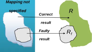
Every item of software at its most primitive level may be viewed as a function or mapping according to some specification, S, from a set of input values (its domain, D) to a set of output values (its range, R).
A program which implements specification S should also map from D to R. However, if a fault f exists in the program, there will be some subset of the domain, Df say, on which the erroneous program Pf computes a faulty result. The set of faulty results, denoted Rf, may contain values both in R and outside R. The effect of Pf on values outside of D remains unspecified. See Figure 1. Note that the domain and the range can be considered for an entire program, an individual program component, a program path or simply a single program location.
3. Domain-to-Range Ratio (DRR)
The domain-to-range ratio (DRR) has been proposed by Voas and Miller [11] as a specification metric. Put sim-
ply:
Domain-to-Range Ratio D R
[image:2.595.326.521.602.713.2] (1)
where |D| is the cardinality of the domain of the specification and |R| is the cardinality of the range. DRR can be determined for mathematical or computational functions. As presented in [10] we consider, for example, the function f(d) = d mod 2, where the input d is a member of the set of natural numbers not greater than 100, i.e. D
1, 2, 3,,100
. Clearly the function generates only two possible outputs, namely 0 when d is even and 1 when d is odd, so that R = {0,1} and DRR = 100/2 = 50. Difficulties arise when the domain and the range, are infinite.DRR metric provides an approximate measure of in- formation loss. Information loss may become manifest as “internal data state collapse” which occurs when two dif- ferent data states are input in a program and produces the same output state. Voas and Miller [11,12] remark a connection between DRR and state collapse as presented [10], and imply that the testability of a program is corre- lated with the DRR. High DRR is thought to lead to low testability and vice versa.
4. Domain Testability and DRR
Domain testability involves use of the concepts of obser- vability and controllability [5]. A software component is observable, if a test input is repeated, the output is the same. If the outputs are not the same, the component is dependent on hidden states not identified by the tester and Freedman calls this an “input inconsistency”. A soft- ware component is controllable, if an output identifier is specified to be a certain range of values and there are particular instances of values that cannot be generated by any test input values, those are termed “output inconsis- tencies”.
Most functions and procedures are not a priori observable and controllable. The modifications required to achieve domain testability are called extensions.
R
R
f Faultyresult Correct
result
Mapping not
specified
Observable extensions are achieved by introducing new input variables so that the component becomes observa- ble, i.e. distinct outputs can only arise from distinct inputs.Controllable extensions are achieved by modify- ing outputs for the given component so that it becomes controllable, i.e. all claimed outputs are attainable with some input. Controllability is achieved by an appropriate reduction of the range. Observability and Controllability can be measured as presented in [10].
In order to consider the relationship between domain testability and domain-to-range ratio, the domain and range of the component after modification with observ- able and controllable extensions can be written as [10]:
DRR D D D
R R R
(2)
Domain-to-range ratio of a program component, after modification to make it domain testable, is the domain- to-range ratio of the component before modification mul- tiplied by one plus the relative size of the domain exten- sion and divided by one minus the relative size of the range reduction.
5. Semantic Fault Size
Offutt and Hayes [13] drew a distinction between the syntactic and the semantic nature of faults. The syntactic nature can be described by the syntactical differences between the faulty program and the correct program. The semantic nature of a fault, on the other hand, results from the view that for some subset of the input domain a faulty computation takes place producing incorrect output. Corresponding to the syntactic size of a fault, Offutt and Hayes defined the semantic size of a fault as “the relative size of the sub domain of D for which the output map- ping is incorrect”. It should be obvious that there is no reason why there should be a link between syntactic fault size and semantic fault size. Indeed it is perfectly possi- ble to find situations where a syntactically small fault results in a very large semantic fault size, and vice versa.
5.1. Semantic Fault Size and Testability
Offutt and Hayes [13] suggested that semantic fault size is closely related to testability in the sense of Voas et al. [6]. If a statement in the subject program has low testability, then any fault associated with that statement might be expected to have small semantic size and any statement containing a fault with large semantic size could be expected to exhibit high testability.
To explore this connection between semantic size and testability further, consider the propagation, infection and execution (PIE) model that provides the basis for test- ability estimation. According to the PIE model, the probability of failure under a particular input distribution,
is a combination of the individual probabilities: 1) that the fault is executed (E = execution); 2) that execution of the fault causes corruption of the data state (I = infection); and 3) that the faulty data state propagates to the output (P = propagation) [14].
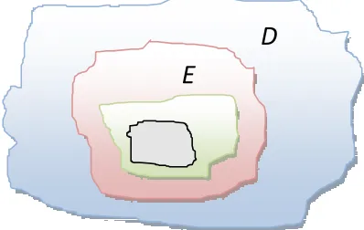
Referring to Figure 2, where, as before, D represents the entire input domain of the subject program, there will be some subset E of D such that all test values in E cause the fault to be executed. Amongst those input values that cause fault execution, some will result in data state infection, as represented by the region I. Finally amongst those input values that cause data state infection, some will propagate the faulty state to the output, as repre- sented by the region P.
In practice Voas [9] suggests estimating testability at a location by separate estimation processes for the three individual components of the model. These processes are presented in Section 6.
An alternative testability estimation procedure could be based on considering versions of the chosen program with location L mutated. The mutation change, provided it does not generate an equivalent mutant, can be regarded as a seeded fault that has a semantic size in the same way as naturally occurring faults. The smallest semantic size of such mutants, being a worst case, could provide an estimate for testability at the location L.
A traditional (strong) mutation testing tool such as Mothra [14] could be used. It requires establishing a large number of input test cases chosen randomly from the input domain and then determining for each mutant generated by the tool, the proportion of test cases that kill that mutant. This is different from normal usage where, once a mutant is killed with some test case, no further test cases are applied to that mutant. Offutt and Hayes [13] did adopt this procedure to estimate the semantic size of all mutants created by the same mutation operator in an attempt to measure the size of given fault types. The aim is to determine the minimum semantic size of all mutations at a location. Although still an expensive process, this has the merit, superficially at least, of being considerably more straightforward than using separate
E
[image:3.595.323.522.592.718.2]D
estimation procedures for the three components of the PIE model.
It is noted in passing that since propagation analysis is akin to strong mutation testing, and infection analysis is akin to weak mutation testing, a similar distinction could be made for semantic fault size. On the other hand, weak semantic fault size can be considered as the proportion of the input domain that merely results in an infected data state immediately after executing a fault, i.e.
Weak semantic fault size I
D
(3)
5.2. Semantic Fault Size and DRR
Semantic can be related to the domain-to-range ratio (DRR). However, since semantic fault size depends solely on the input domain, whereas DRR depends on both the domain and the range, there is unlikely to be a direct connection. What can be deduced is a relationship involving fault size, measured in terms of input and output, and DRR both for the correct program and also for a faulty version when executed over just that portion of the domain that exposes the fault.
Then denoting DRR for the correct program P with input domain D by DRRPD and for faulty program Pf with just the fault-exposing input domain Df by
DRR
fDf
P the following is obtained:
output fault size
DRR DRR
input fault size
f f
D D
P P (4)
This equation captures the (admittedly) rather limited connection between DRR and semantic fault size.
6. The Process Meta-Model
Process modeling is considered today as a key issue by both the Software Engineering (SE) and the Information Systems Engineering (ISE) communities. Recent interest in process modeling is part of the shift of focus from the product to the process view of systems development. There is already considerable evidence for believing that there shall be both: improved productivity of the soft- ware systems industry and improved systems quality, as a result of improved development processes. Recent in- depth studies of software development practices [15], however, demonstrate that we know very little about the development process. Thus, to realize the promise of systems development processes, there is a great need for “a conceptual process model framework” [16].
Process modeling is a rather new research area. Con- sequently there is no consensus on what is a good for- malism to represent processes or even on what the final objectives [15]. Process models may be constructed for a number of different reasons, to fulfill different purposes.
One purpose may be purely descriptive, that is, to record how some process or class of processes is actually per-formed.
Alternatively, models may be constructed to guide, support and provide advises or instructions to developers, i.e.: to be prescriptive. The SE community has focused on descriptive models more than the ISE community.
Yet another way of looking at process models is in terms of the process aspect that they address: some focus on managerial aspects of the development process where- as others have technical concerns.
We propose in this paper a well-defined and repeatable approach to generate well-formed guidance centered process models. For guidance centered process models to be well-formed, we have identified a list of requirements and intentions.
To realize and adapt this approach we adopted a goal- perspective, the Map-driven process modeling approach. The Map approach is a representation system based on intentions and strategies. In this system, intentions ab- stract from organizational tasks and the different ways in which tasks are performed are intention-achievement strategies. The map is capable of abstracting from the detail of business processes to highlight organizational goals and their achievement.
In this section we first introduce the key concepts of a map and their relationships. Then we define map com- ponents as process to for modeling the testability process.
The Process Meta-Model Formalized with MAP
This process is modeled using MAP formalism which is a process model. This model is a process representation system based on a non-deterministic ordering of goals and strategies [17]. A map can be represented as a la- beled directed graph. The nodes represent goals and the links between nodescorrespond to strategies. The di- rected nature of the graph shows the order of the differ- ent goals.
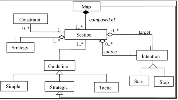
A MAP is defined as a meta-process model which al- lows designing several processes under a single repre- sentation (Figure 3). It is a labeled directed graph with intentions as nodes and strategies as edges between in- tentions. A MAP is composed of one or more sections. A section is a triplet < source intention I, target intention J, strategy Sij> that captures the specific manner to achieve the intention J starting from the intention I with the strategy Sij. An intention is expressed in natural language and is composed of a verb followed by parameters. Each MAP has two special intentions “Start” and “Stop” to respectively begin and end the navigation in the MAP. Each intention can only appear once in a given MAP. Each section is associated a guideline that can be one of the following three types: Simple, Tactic or Strategic.
Figure 3. The MAP process meta-model.
SSG and ISG. IAG can be one of the aforementioned types namely tactic or simple or strategic while SSG and ISG are always tactic guidelines. For more details see [18]. These guidelines are further explained below.
1) A guideline named “Intention Achievement Guide- line” (IAG) is associated to each section providing an operational mean to satisfy the target intention of the section.
2) “Strategy Selection Guideline” (SSG) determines which strategies connect two intentions and helps to choose the most appropriate one according to the given situation. It is applied when more than one strategy exists to satisfy a target intention from a source one.
3) “Intention Selection Guideline” (ISG) determines which intentions follow a given one and helps in the se-lection of one of them. It results in the selected intention and the corresponding set of either IAGs or SSGs. The former is valid when there is only one section between the source and target intentions, whereas the latter occurs when there are several sections.
Figure 4 shows that: 1) for a section <Ii, Ij, Sij>, there is an IAG, 2) for a couple of intentions <Ii, Ij>, there is an SSG, and 3) for an intention Ii, there is an ISG.
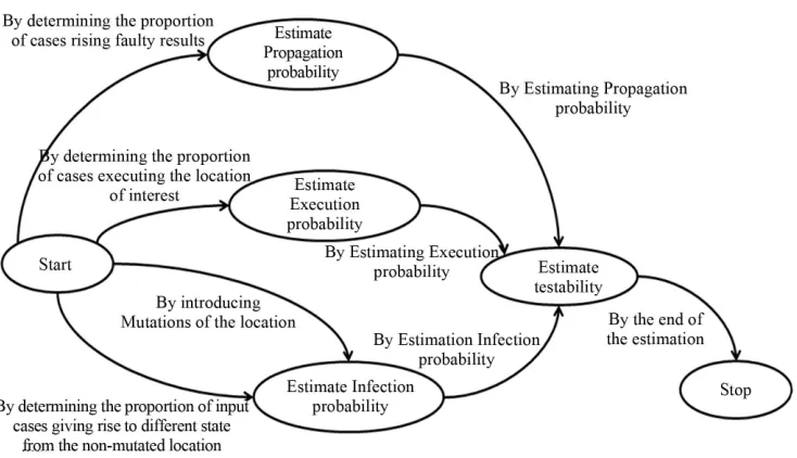
As presented in Figure 5, a map has two special goals, Start and Stop which represent the beginning and the ending of the process respectively. A goal represents a state that is expected to be reached and a strategy corre- sponds to how to achieve a goal. To estimate the testabil- ity, the process consists of the estimation of the probabil- ity of propagation, infection and execution. We try through this MAP to model our process. We can find the principal goals which are the estimation of the probabil- ity of propagation, infection and execution. Achieving these goals allows the estimation of the testability.
Also, the process meta-model for the Testability for- malized using MAP is shown in Figure 5. It contains four core intentions “Estimate Propagation probability” and “Estimate Execution Probability”, “Estimate Infec-
tion Probability” and “Estimate Testability” in addition to “Start” and “Stop” intentions. We use also this process model to elaborate and to present the relationship be- tween testability, PIE, DRR and semantic fault size as presented in Figure 6. The main purpose of using the MAP formalism is to simplify the relationship between testability (PIE), DRR and semantic fault size. The MAP model was introduced in this paper in order to model processes in a flexible way.
To allow tester or user to go through the different intentions of the map, the approach provides a set of factors called Situational Factors [19,20].
Estimating testability involves the use of observability, controllability concepts and some extensions which are modifications required to achieve domain testability. The relationship between testability and semantic fault size is important where in case of low testability we expect to have small semantic size and in case of high testabilitywe expect to have large semantic fault size. Testability is correlated with the domain/range ratio. Adapting do- main-to-range ratio needs two ways: to invert the ratio so that it becomes the range-to-domain ratio (RDR) or to calculate the range-to-domain ratio dynamically.
The proposed situational factors characterize current situation and then, help designer to choose the appropri- ate strategy among several presented in the map. We have identified the following factors: Application type, Application complexity, Similarity with others applica- tions, User-application adaptation, User-application adaptation, Tester Experience [7].
Situational factors guide and orient tester during test- ing through the design meta-model process. When we say guide the tester we mean that this person can choose the appropriate goal to achieve the different options in PIE process (propagation estimation, infection estima- tion and execution estimation). After the achievements of these goals, the tester can calculate the global test-
Figure 4. Guidelines associated with the MAP.
Figure 5. Testability Process Modeled using MAP formalism.
7. Other Related Work
This section briefly mentions some of the most signi- ficant related work (besides that already cited) which is concerned with fault models, fault propagation and fault- based testing.
The PIE model bears some similarity to the RELAY model [21] in which a fault originates a potential failure that must then transfer through computations to produce a state failure and ultimately be revealed as an external failure. Morell [22] developed a theory of fault-based testing that placed emphasis on fault propagation and then used symbolic testing to explore its limitations. The work of Goradia [23] was also concerned with fault propagation and a technique known as “dynamic impact
analysis” was formulated to determine the extent of the effect of program components on the program output for a specific test case. Hamlet and Voas [24] showed just how useful a PIE testability estimate could be when used in conjunction with conventional reliability testing to provide, via so-called “squeeze play”, a confidence bound for the correctness of a program. On a more cau- tionary note however, they also provided a stark critique of the assumptions underlying the PIE model.
[image:6.595.117.484.322.533.2]Figure 6. Relationship between testability, DRR and semantic fault size.
defined in [18] and has been the subject of many uses that go beyond the representation of process engineering. We can find for example the use of maps for require- ments engineering and alignment of COTS products or customization of an ERP system to the needs of an organization [25-27].
Finally to validate our proposed approach, we have focused, after that, in describing how the approach guides through an empirical evaluation.
8. Conclusions
Testability is an important attribute of software as far as the testing community is concerned since its measure- ment leads to the prospect of facilitating and improving the testing process. Unfortunately testability has various guises. Two distinct and significant interpretations are due to Freedman [5] and Voas et al. [6]. Freedman’s notion of testability has two facets, observability and controllability, both of which can be measured by the extent of certain modifications to a program component. Voas’s notion of testability can be estimated by the com- putationally expensive PIE technique and Voas himself has suggested a possible link with the rather simpler con- cept of domain-to-range ratio.
By taking a functional view of software, this paper has produced a succinct characterization of controllability and observability and developed a simple mathematical relationship involving them and the domain-to-range ratio. Semantic fault size has also been considered and its relationship with Voas’s testability has been explored. A consequence of this is the suggestion that testability of a program location could be estimated more straightfor- wardly by a small adaptation of the traditional strong
mutation testing process, to find the minimum semantic size of all mutants at the location. Finally some refine- ments of semantic fault size have been introduced and their relationship with DRR has been considered. To visualize the PIE model, we model the process using the system of representation MAP. This formalism allows giving more importance to the goals and the strategies used in this process.
The authors recognize the desirability of validating the connections between the concepts as discussed here. Validation could take the form of empirical evidence, but could also consider a more analytical approach along the lines adopted by How Tai Wah [28-30] who has modeled software as finite functions to deduce theoretical results concerning fault coupling. In the meantime, this paper has made a limited start at putting together the various separate pieces of what might be considered a rather complex jigsaw of related concepts.
REFERENCES
[1] R. Bache and M. Müllerburg, “Measures of Testability as a Basis for Quality Assurance,” Software Engineering Journal, Vol. 5, No. 2, 1990, pp. 86-92.
http://dx.doi.org/10.1049/sej.1990.0011
[2] J. Bainbridge, “Defining Testability Metrics Axiomati- cally,” Software Testing, Verification and Reliability, Vol. 4, No. 2, 1994, pp. 63-80.
http://dx.doi.org/10.1002/stvr.4370040203
[3] A. Bertolino and L. Strigini, “On the Use of Testability Measures for Dependability Assessment,” IEEE Transac- tions on Software Engineering, Vol. 22, No. 2, 1996, pp. 97-108.
Evaluation of Software Quality,” Proceedings of 2nd In-ternational Conference on Software Engineering, San Francisco, IEEE Press, 1976, pp. 592-605.
[5] R. S. Freedman, “Testability of Software Components,”
IEEE Transactions on Software Engineering, Vol. 17, No. 6, 1991, pp. 553-564.
[6] J. M. Voas, L. J. Morell and K. W. Miller, “Predicting Where Faults Can Hide from Testing,” IEEE Software, Vol. 8, No. 2, 1991, pp. 41-48.
http://dx.doi.org/10.1109/52.73748
[7] J. Gao, J. Tsao and Y. Wu, “Testing and Quality Assu- rance for Component-Based Software,” Artech House, 2005.
[8] N. Kazuteru, “Delay Fault Testability on Two-Rail Logic Circuits,” Proceeding of the Defect and Fault Tolerance of VLSI Systems, DFTVS ‘08. IEEE International Sympo-sium, Boston, 1-3 October, 2008, pp. 482-490.
[9] J. M. Voas, “PIE: A Dynamic Failure-Based Technique,”
IEEE Transactions on Software Engineering, Vol. 18, No. 8, 1992, pp. 717-727.
[10] M. R. Woodward and Z. A. Al-Khanjari, “Testability, Fault Size and the Domain-to-Range Ratio: An Eternal Triangle,” Software Engineering Notes, Vol. 25, No. 5, 2000, pp. 168-172.
http://dx.doi.org/10.1145/347636.349016
[11] J. M. Voas and K. W. Miller, “Semantic Metrics for Soft- ware Testability,” The Journal of Systems and Software, Vol. 20, No. 3, 1993, pp. 207-216.
http://dx.doi.org/10.1016/0164-1212(93)90064-5
[12] M. R. Woodward and Z. A. Khanjari, “Testability, Fault Size and the Domain-to-Range Ratio: An Eternal Trian- gle,” Proceedings of the ACM SIGSOFT International symposium on Software Testing and Analysis, Vol. 25, No. 5, 2000. pp. 168-172.
[13] A. J. Offutt and J. H. Hayes, “A Semantic Model of Pro-gram Faults,” Proc. Int. Symp. on Software Testing and AnalysisISSTA ’96, San Diego, ACM Press, 1996, pp. 195-200.
[14] R. A. DeMillo, D. S. Guindi, W. M. McCracken, A. J. Offutt and K. N. King, “An Extended Overview of the Mothra Software Testing Environment,” Proc. Second Workshop on Software Testing, Verification and Analysis, Banff, IEEE Press, 1988, pp. 142-151.
http://dx.doi.org/10.1109/WST.1988.5369
[15] M. A. Friedman and J. M. Voas, “Software Assessment: Reliability, Safety, Testability,” Wiley, New York, 1995. [16] N. Kraiem, “Use of the Process Meta-Model to Describe
Requirements Engineering Methodologies,” Proceeding of the ICECCS, Como, 1997, pp. 306-318.
[17] S. Selmi, N. Kraiem and H. Hajjami Ben Ghazala, “WApDM: A Multi-Process Approach for Web Applica- tions Design,” Proceedings of International Conference on Internet Computing ICOMP’05, Las Vegas, June 27- 30, 2005, pp. 115-125.
[18] C. Rolland and N. Prakash, “On the Adequate Modeling of Business Process Families,” Proceedings of 8th Work- shop on Business Process Modeling, Development, and Support (BPMDS’07) Norway, 2007, pp. 1-8.
[19] C. Rolland, N. Prakash and A. Benjamen, “A Multi- Model View of Process Modelling,” Requirements Engi- neering, Vol. 4, No. 4, 1999, pp. 169-187.
http://dx.doi.org/10.1007/s007660050018
[20] S. S. Selmi, N. Kraiem and H. H. Ben Ghezala, “Guidan- ce in Web Applications Design,” Proceeding of the MoDISE-EUS’08 (CAISE2008), Montpellier, June 2008, pp. 114-125.
[21] D. J. Richardson and M. C. Thompson, “An Analysis of Test Data Selection Criteria Using the RELAY Model of Fault Detection,” IEEE Transactions on Software Engi-neering, Vol. 19, No. 6, 1993, pp. 533-553.
[22] L. J. Morell, “A Theory of Fault-Based Testing,” IEEE Transactions on Software Engineering, Vol. 16, No. 8, 1990, pp. 844-857.
[23] T. Goradia, “Dynamic Impact Analysis: A Cost-Effective Technique to Enforce Error-Propagation,” Proc. Int. Symp. on Software Testing and Analysis ISSTA ’93, Cambridge, ACM Press, 1993, pp. 171-181.
[24] D. Hamlet and J. Voas, “Faults on Its Sleeve: Amplifying Software Reliability Testing,” Proc. Int. Symp. on Soft-ware Testing and AnalysisISSTA ’93, Cambridge, ACM Press, 1993, pp. 89-98.
[25] C. Rolland and N. Prakash, “Bridging the Gap between Organisational Needs and ERP Functionality,” Require-ments Engineering Journal, Vol. 5, 2000, pp. 180-193. [26] C. Rolland and N. Prakash, “Matching ERP System
Functionality to Customer Requirements,” Proceedings of the 5th IEEE International Symposium on Requirements Engineering, Toronto, August 27-31, 2001, pp. 66-75. [27] C. Rolland, C. Salinesi and A. Etien, “Eliciting Gaps in
Requirements Change,” Requirements Engineering Jour- nal, Vol. 9, No. 1, 2003, pp. 1-15.
[28] C. Rolland and C. Salinesi, “Fitting Business Models to Systems Functionality Exploring the Fitness Relation-ship,” Proceedings of the 15th Conference on Advanced Information Systems Engineering CAiSE’03, Austria, June 2003, pp. 647-664.
[29] K. S. How Tai Wah, “A Theoretical Study of Fault Cou- pling,” Software Testing, Verification and Reliability, Vol. 10, No. 1, 2000, pp. 3-45.
http://dx.doi.org/10.1002/(SICI)1099-1689(200003)10:1< 3::AID-STVR196>3.0.CO;2-P