© 2017, IRJET | Impact Factor value: 5.181 | ISO 9001:2008 Certified Journal
| Page 1443
QSAR studies of breast carcinoma using Artificial neural network,
Bayesian classifier and Multiple linear regression
Guru Pratap Singh, Rajnish Kumar, Anju Sharma
Amity Institute of Biotechnology, Amity University Uttar Pradesh, Lucknow Campus, Lucknow- 226010,
Uttar Pradesh, India
---***---Abstract -
Breast cancer is a disease that affects millions. Itstarts as a tumor but end up spreading all over the body. It uses nutrition of body for its own growth and there is no regulatory mechanism for its growth. Breast cancer has no cure once it progresses to an advanced stage. Therefore, it is very crucial to detect the breast cancer at early stage. An attempt has been made to develop a prediction model for breast cancer to find out the malignancy of a tumor using machine learning algorithms of artificial intelligence. Artificial neural network (ANN), Bayesian classifier and Multiple linear regression (MLR) were used to generate the prediction models using a dataset of 699 patients. Descriptors used to generate prediction models were uniformity of cell size, bare nuclei, bland chromatin and normal nucleoli. The percentage accuracies of generated models for ANN, Bayesian classifier and MLR were found to be 83.73%, 83.53% and 82.14% respectively. These models can potentially be useful for preliminary classification of breast cancer.
Key Words: QAR, ANN, Breast cancer, MLR
1.INTRODUCTION
Ductal carcinoma is most common categories of breast cancer. Breast cancer initiates in lobulous cells. Invasive breast cancer spreads from the point of initiation to the surrounding tissues. Breast cancer can occur in both females and males which opposes the common orthodox belief that it occurs only in females [1].
1.1 Types of breast cancer 1.1.1 Ductal carcinoma in situ
It is a non-invasive cancer where in the lining of breast milk duct abnormal cells have been found. It is treatable in the initial stage but if ignored it can spread in surrounding tissue [2].
1.1.2 Invasive ductal carcinoma
Here, abnormal cells spread out side of the duct area into other parts. There is a possibility that it may spread in other body parts. It is also known as ductal carcinoma. It’s the most common type of breast cancer makes (about 70% of all cases) and it also most commonly affects males [3]. 1.1.3 Triple negative breast cancer
It occurs due to absence of the three receptors that provide the fuel for most breast cancer growth like progesterone, estrogenandher-2/neu gene in cancer tumours. Due to this the breast cancer cannot be treated with common hormone
therapy as it lacks all the above mentioned hormone, but drug therapy or chemotherapy is proven to be effective for this type of cancer [4].
1.1.4 Inflammatory breast cancer
In this category of breast cancer, tumor cells attack the lymph vessels and skin of the breast. This cancer lacks distinct tumor or lymph that can be felt or isolated. Symptoms begin to appear when lymph vessels are blocked by cancer cells. [5] Common symptoms are basically of three types:
(a) Breast may be swollen, warm and red
(b) Skin surrounding breast may appear like orange peel (c) Nipple develops inversion, flattening and dimpling may occur
1.1.5 Metastatic breast cancer
It is called stage four breast cancer where it spreads to other parts of the body which includes lungs, liver, brain and bones. It develops or spreads by invading nearby healthy cells, penetrating into lymphatic system and circulatory system after that they migrate through circulatory system, cancer cells gets lodged into capillaries, last step includes growth of new small tumor.
1.1.6 Breast cancer during pregnancy
Any type of cancer that occurs during pregnancy comes under this category
1.1.7 Medullary carcinoma
It accounts for about 3 to 5 percent of all types of breast cancer tumors appear on mammogram, but they don’t necessarily feel like a lump it may appear like a spongy change of breast tissue.
1.1.7 Tubular carcinoma
Its occurrence is about 2%. This type of cancer has a distinctive tubular structure when viewed under microscope, it can be found by a mammogram and it feels spongy. Found in women around 50 and above can be treated by hormone therapy [6].
1.1.8 Mucinous carcinoma
This type of carcinoma occurs in 1 to 2 percent of all the cases. Here cells produce mucus and are poorly defined. 1.1.9 Paget disease of the breast or nipple
It is also known as paget disease, rare cancer affects skin of the nipple and often areola. It is misdiagnosed because its symptoms are confused with common skin conditions. 1.2 Frequently used computational approaches for classification of biological data
1.2.1 QSAR Modelling
© 2017, IRJET | Impact Factor value: 5.181 | ISO 9001:2008 Certified Journal
| Page 1444
model is improved by adding and removing descriptors afterthis mathematical equation is also improved.[7] Three basic requirement for QSAR Model Generation are as follow: •Each data set should represent a particular biological activity.
•We should have structures of molecules so as to predict a particular biological activity.
•We should have a statistical software which supports the values of descriptors of present in statistical manner. 1.2.2 Artificial Neural Network (ANN)
Neural network is a human brain based reasoning model. Brain contains neurons that are fundamental unit of biological neural network, a neuron contains soma, dendrites and axons.
Artificial neural network consists of numerous simple processors called neurons, analogous to biological neurons. Here weighted links connect neurons that pass the signal form one neuron to another. [8]
Similarities of biological neurons and artificial neural network are;
Biological neural network Artificial neural network
Soma Neuron
Dendrite Input
Axon Output
Synapse Weight
The output signal is transferred through the outgoing connection of neuron. The outgoing connection divide into numerous branches that transmit the same signal. These outgoing branches end at the incoming connections of other neurons in the network.
Neuron computes the weighted sum of input signals and it also compares the result with a special value called threshold value denoted by q.
If threshold is greater than the net input, the neuron output will be –1. But if threshold is lower or equal to net input, the neuron is activated and its output becomes +1.
Activation function:
X = wixi Y = +1 if X ≥ θ -1 if X ≤ θ
This type of activation function is called a sign function. Perceptron
It is a feed forward neural network of simple kind: a linear classifier. Perceptron is a classifier of binary type that maps its input x vector to an output value f(x)
f(x)= 1 if w*x +b>0 0 else
Where w* x is the dot product and a vector of real-valued weights is w. b is the 'bias', a constant term that does not depend on any input value.
Binary classification problem: The value of f(x) (0 or 1) is used to classify x as either a negative or a positive instance.
As output feed directly on input unit via the weighted connections, the perceptron is considered a feed-forward neural network of the simplest kind.
Perceptron’s training algorithm
Step 1: Initialisation
Setting of initial weights w1, w2,…, wn and threshold q to random numbers in the range [-0.5, 0.5]. If the error, e(p), is negative, we need to decrease Y(p) but if it is positive, we need to increase perceptron output Y(p)
Step 2: Activation
Activate the perceptron by applying desired output Yd (p) and inputs x1(p), x2(p),…, xn(p). Calculate the actual output at p = 1
Where step is a step activation function and n is the number of the perceptron inputs.
Step 3: Weight training
Update the weights of the perceptron where ∆wi(p) is the weight correction at iteration p.
The weight correction is computed by the delta rule: Step 4: Iteration
Increase iteration p by one, go back to Step 2 and repeat the process until convergence.
Two dimensional plots of basic logical operations. [9]
Multilayer Neural Networks
A multilayer perceptron is just like simple perceptron with one or more hidden layers. The network contains an input layer of source neurons, at least one hidden layer or middle of computational neurons as well as an output layer of computational neurons.
The input signals are propagated on a layer-by-layer basis in forward direction (figure 1). A hidden layer “hides” its output that is desired by us. Neurons of hidden layer can't be observed through the input as well as the output behaviour of the network.
ANN can have n number of hidden layers and n number of input nodes. Each layer can sustain from 10 to 1000 neurons. An experimental neural networks can have six or even seven layers, including four or five hidden layers, and utilise millions of neurons.
[image:2.595.350.522.658.724.2]Learning process for a multilayer network proceeds in the same way as for a perceptron. A training set containing input patterns is presented to the network. The network computes its output pattern, and in case of an error or in other words there is a difference between desired and actual output patterns. The weights are then adjusted to reduce or eliminate this error. [10]
Figure 1: Showing arrangement of layers in multilayer ANN Back-propagation in ANN
Input layer
First hidden
layer
Second hidden layer
Output layer
O
u
t p
u
t
S
i g
n
a
l s
I n
p
u
t
S
i g
n
a
l
© 2017, IRJET | Impact Factor value: 5.181 | ISO 9001:2008 Certified Journal
| Page 1445
In back-propagation of neural network, here the learningalgorithm has two parts. First, we present a training input pattern to the network input layer. Then the network propagates the input pattern from one layer to another layer until the output layer generates the output pattern. If the obtained pattern is different from the desired output then the error will be calculated and propagated backwards through network from output layer to input layer. As the error is propagated the weights are modified.
1.2.3 Bayesian Logic
It is a means to quantify uncertainty. It is based on probability, it refines a hypothesis by factoring background information and additional information which leads to a number of representations that the probability may be true or the hypothesis may be true. [11]
Bayesian Theory
Let the class label of a data sample X be unknown. Here let H be some hypothesis that X belongs to some class C. For instance we want to determine P(H/X) that is our hypothesis H holds for X which is the observed data.
P(H/X)=P(X/H)P(H)
P(X)
1.2.4 Multiple regression
It finds a relationship between two or more variables and response variable by filtering equation (linear equations) to the data we have observed. Let us assume we have two variables x and y where every value of independent variable y is associated with variable x
Where c, m1, m2, m3,…, mm are coefficients and x1, x2, x3,……..xn are descriptor values and n is number of molecules
Where y is scalar quantity and represent activity, xi is value of descriptor, where i and mi is its associated coefficient and c is the intercept or error[12].
2. Material and Method
2.1 Study Prerequisites
Weka tool: It is a tool with machine learning algorithms and data mining facilities. These algorithms can be directly applied to a data set or can be applied on a data code created by the user e.g. Java code. Weka contains tools for data classification, pre-processing, association rule, clustering and visualization. It can also be used for creation of new machine learning schemes.
2.2 Data Preparation
2.2.1 Training Set and Test Set
Data set used in this study was collected from UCI machine learning repository.[13] Classification of data was done into test and training data. Division was done on the random basis where 75% of data was taken for training set and 25% was used as test data. [14] There were only two class
attributes benign and malignant, so separate 3:1 division was done for both the classes. Total data we had was of 699 patients, data contains 9 descriptors and 2 classes. The descriptors used in current study were Clump Thickness (Clump), Uniformity of Cell Size (Ucellsize), Uniformity of Cell Shape (Ucellshape), Marginal Adhesion (Mgadhesion), Single Epithelial Cell Size (Sepics), Bare Nuclei(Bnuclei), Bland Chromatin (Bchromatin), Normal Nucleoli(Normnucl), Mitosis (Mitoses). The two classes were benign and malignant. After division we had 504 of training data and 195 of test data. Training set contained 101 malignant and 403 benign data. Test set contained 62 malignant and 133 benign data.
2.2.2 Normalization
Normalization provides a fine balance of the influence of descriptor when they are combined together. It is also crucial as, it is required as descriptor usually represents a wide range of physio-chemical properties. If values do not lie within a particular range of all the descriptors then a possibility may exist that descriptor with large range of values dominate the descriptor selection process as well as modelling process, thus a model will be generated which will be biased to a particular property. Therefore in order for such a problem to be avoided we need to calibrate the descriptors values by bringing them into the same range. Normalization was done using standard deviation method. 2.2.3 Standard deviation: Mean and standard deviation is calculated for each and every descriptor. Descriptors are scaled using following equation: [15]
x
deviation
dard
s
x
mean
x
x
ii
_
tan
'
2.3 Descriptor Selection
Descriptor selection is critical for two reasons. First, to reduce the computationally expensive calculations and second, to minimize the effect of higher values on lower values. Here, two methods were used; manual selection method and automated methods which include correlation matrix and BestFit & CfsS, Ranker+ One R Attribute Eval with combination of Ranker-Symmetrical Uncert Attribute Eval respectively.
2.3.1 Co-relation matrix
This matrix was generated between all the descriptors and classes as a result it was 11*11 matrix. Class labels were placed for normalized values i.e. benign was represented by class level zero and of malignant class label one was considered. We checked the maximum similarity of all the descriptors with class and then we selected the descriptors. Among the selected descriptors, internal similarities between descriptors were considered and those with maximum similarities were evaluated on the basis of their internal similarities and the similarities of the class (figure 2).
n
i mixi c
© 2017, IRJET | Impact Factor value: 5.181 | ISO 9001:2008 Certified Journal
| Page 1446
clump ucellsize ucellshape mgadhesion sepics bnuclei bchromatin normnucl mitoses class
clump 0 0.609 0.617 0.457 0.469 0.569 0.535 0.556 0.345 0.459
ucellsize 0.000 0.899 0.715 0.699 0.673 0.743 0.732 0.450 0.529
ucellshape 0.000 0.679 0.668 0.699 0.728 0.732 0.438 0.539
mgadhesion 0.000 0.589 0.668 0.657 0.613 0.442 0.413
sepics 0.000 0.555 0.581 0.628 0.490 0.432
bnuclei 0.000 0.664 0.603 0.352 0.528
bchromatin 0.000 0.669 0.375 0.472
normnucl 0.000 0.433 0.514
mitoses 0.000 0.206
class 0.000
Figure 2: Correlation matrix of collected descriptors. Highlighted descriptors were found to have good correlation with their respective classes.
2.3.2 BestFit and CfsS
Searches the space of attribute subsets by greedy hill climbing augmented with a backtracking facility. Setting the number of consecutive non-improving nodes allowed controls the level of backtracking done. Best first may start with the empty set of attributes and search forward, or start with the full set of attributes and search backward, or start at any point and search in both directions (by considering all possible single attribute additions and deletions at a given point)
Evaluates the worth of a subset of attributes by considering the individual predictive ability of each feature along with the degree of redundancy between them.
Subsets of features that are highly correlated with the class while having low inter correlation are preferred.
2.3.3 Ranker+OneRAttributeEval
Evaluates the worth of an attribute by using the OneR classifier
2.3.4 Ranker+ Symmetrical Uncert Attribute Eval Evaluates the worth of an attribute by measuring the symmetrical uncertainty with respect to the class.
SymmU(Class, Attribute) = 2 * (H(Class) - H(Class | Attribute)) / H(Class) + H(Attribute).
Results of descriptor selection methods are summarised in Table 1.
Table 1: Selected descriptors from automatic and manual descriptor selection methods
Method Selected descriptor
Correlation matrix Ucellshape, Bnuclei, Bchromatin, Normnucl
BestFit and CfsS Clump, Ucellshape, Mgadhesion, Sepics, Bnuclei, Bchromatin, Normnucl
Ranker+OneRAttribute
Eval Normnucl, Mgadhesion, Ucellsize, Ucellshape, Clump, Sepics, Bnuclei, Bchromatin, Mitisos Ranker+ Symmetrical
Uncert Attribute Eval Ucellshape, Normnucl, Sepics, Bnulei, Ucellsize, Bchromatin, Mgadhesion, Clump, Mitosis
Finally, four common descriptors were selected. Selected descriptors were Ucellshape, Bnuclei, Bchromatin and Normnucl.
3. Prediction models generation
Prediction models were generated using ANN, Bayesian classifier and multiple linear regression using common descriptors selected from various manual and automated descriptor selection methods. The training sets were used to generate prediction models and independent test sets were used to check the accuracy of generated models.
4. Results and Discussion
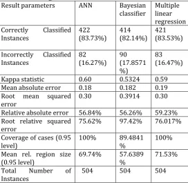
[image:4.595.36.300.101.251.2]The training dataset, results of ANN and MLR were found to be comparative. Prediction models generated using ANN and MLR were able to correctly classify the instances with accuracy of 83.73% and 83.53% respectively for training set. However, Bayesian classifier found to be slightly inferior and yielded 82.14% accuracy while classifying the instances for training set. Detailed results for training set are summarised in Table II.
Table II: Training Dataset results
Result parameters ANN Bayesian
classifier Multiple linear regression Correctly Classified
Instances 422 (83.73%) 414 (82.14%) 421 (83.53%)
Incorrectly Classified
Instances 82 (16.27%) 90 (17.8571 %)
83 (16.47%)
Kappa statistic 0.60 0.5324 0.59 Mean absolute error 0.18 0.182 0.19 Root mean squared
error 0.30 0.3914 0.30 Relative absolute error 56.84% 56.26% 59.23% Root relative squared
error 75.62% 97.42% 76.017% Coverage of cases (0.95
level) 100% 89.4841 % 100% Mean rel. region size
(0.95 level) 69.74% 57.6389 % 71.53% Total Number of
Instances 504 504 504
[image:4.595.307.580.361.626.2]© 2017, IRJET | Impact Factor value: 5.181 | ISO 9001:2008 Certified Journal
| Page 1447
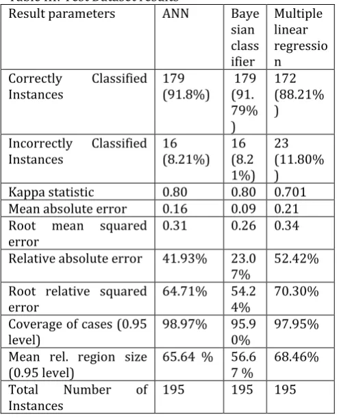
Table III: Test Dataset resultsResult parameters ANN Baye sian class ifier
Multiple linear regressio n Correctly Classified
Instances 179 (91.8%) 179 (91. 79% )
172 (88.21% )
Incorrectly Classified
Instances 16 (8.21%) 16 (8.2 1%)
23 (11.80% ) Kappa statistic 0.80 0.80 0.701 Mean absolute error 0.16 0.09 0.21 Root mean squared
error 0.31 0.26 0.34 Relative absolute error 41.93% 23.0
7% 52.42% Root relative squared
error 64.71% 54.24% 70.30% Coverage of cases (0.95
level) 98.97% 95.90% 97.95% Mean rel. region size
(0.95 level) 65.64 % 56.67 % 68.46% Total Number of
Instances 195 195 195
Result analysis of various parameters of three robust machine learning tools i.e. ANN, Bayesian classifier and MLR, it is clearly evident that these tools have similar robustness in classifying the non-linear datasets. However, in terms of accuracy (for training and test set 83.73% and 91.8% respectively) and coverage (for training and test set 100% and 98.97% respectively) , ANN seems to be marginally better then rest of the two.
5. Conclusion
While generating prediction models using three most widely used machine learning methods, it was found that ANN was marginally more accurate for the current data set. However, rest of the two methods i.e. Bayesian classifier and MLR are not far behind in handling non-linear data sets. These machine learning tool have great promises in development of prediction models for breast cancer and can potentially be useful in primary screening of breast cancer types.
REFERENCES
[1] Weigelt B, Geyer FC, Reis-Filho JS. Histological types of breast cancer: How special are they? Molecular Oncology. 2010;4(3):192-208.
[2] Carraro DM, Eliasa EV, Andrade VP. Ductal carcinoma in situ of the breast: morphological and molecular features implicated in progression. Bioscience Reports. 2014;34(1):e00090.
[3] Bhandari V, Gunasekeran G, Naik D, Yadav AK. Infiltrating ductal carcinoma of the breast presenting as breast abscess :
A case report. National Journal of Medical Research. 2013;3(4):422-3.
[4] Verma S, Provencher L, Dent R. Emerging trends in the treatment of triple-negative breast cancer in Canada: a survey. Current Oncology. 2011;18(4):180-90.
[5] Goldfarb JM, Pippen JE. Inflammatory breast cancer: the experience of Baylor University Medical Center at Dallas. Proceeding (Bayl Univ Med Cent). 2011;24(2):86-8. [6] Tekin YB, Guven ESG, Sehitoglu I, Guven4 S. Tubal Pregnancy Associated with Endometrial Carcinoma after In Vitro Fertilization Attempts. Case Reports in Obstetrics and
Gynecology. 2014;1:1-4.
doi:http://dx.doi.org/10.1155/2014/481380.
[7] Cherkasov A, Muratov EN, Fourches D, Varnek A, Baskin II, Cronin M et al. QSAR Modeling: Where Have You Been? Where Are You Going To? Journal of Medicinal Chemistry. 2014;57(12):4977-5010.
[8] Saracoglu ÖG. An Artificial Neural Network Approach for the Prediction of Absorption Measurements of an Evanescent Field Fiber Sensor. Sensors 2008; 8:1585-94. [9] Rosenblatt F. The Perceptron: A Probabilistic Model for Information Storage and Organization in the Brain. Psychological Review. 1958;65(6):386-408. doi: doi:10.1037/h0042519.
[10] Silva LM, Sá JMd, Alexandre LA. Data classification with multilayer perceptrons using a generalized error function. Neural Networks archive. 2008;21(9):1302-10.
[11] Mallick BK, Ghosh D, Ghosh M. Bayesian classification of tumours by using gene expression data. Journal of the Royal Statistical Society: Series B (Statistical Methodology). 2005;67(2):219-34.
[12] Yamanaka N, Okamoto E, Kuwata K, Tanaka N. A multiple regression equation for prediction of posthepatectomy liver failure. Annals of Surgery. 1984;200(5):658-63.
[13] Original Wisconsin Breast Cancer Database [database on the Internet]. UCI machine learning repository. 1992.
Available from:
https://archive.ics.uci.edu/ml/datasets/Breast+Cancer+Wis consin+%28Original%29. Accessed: 3-3-2015
[14] Sharma A, Kumar R, Varadwaj P, Ahmad A, Ashraf G. A comparative study of support vector machine, artificial neural network and bayesian classifier for mutagenicity prediction. Interdisciplinary Sciences: Computational Life Sciences. 2011;3(3):232-9