http://dx.doi.org/10.4236/ijg.2015.63016
Lithological Characterization and Its
Application Based on Three-Dimensional
Structure-Coupled Joint Inversion of Gravity
and Magnetic Data
Junjie Zhou1,2*, Xingdong Zhang1,2, Chunxiao Xiu1,2
1Key Laboratory of Geo-detection (China University of Geosciences, Beijing), Ministry of Education, Beijing,
China
2School of Geophysics and Information Technology, China University of Geosciences, Beijing, China
Email: *[email protected]
Received 10 February 2015; accepted 9 March 2015; published 13 March 2015
Copyright © 2015 by authors and Scientific Research Publishing Inc.
This work is licensed under the Creative Commons Attribution International License (CC BY). http://creativecommons.org/licenses/by/4.0/
Abstract
Incorporating structural-coupling constraint, known as the cross-gradients criterion, helps to im-prove the focussing trend in cross-plot of multiple physical properties. Based on this feature, a post-processing technique is studied to characterize the lithological types of subsurface geological materials after joint inversion. A simple domain transform, which converts two kinds of partici-pant physical properties into an artificial complex array, is adopted to extract anomalies manually from homogenous host rock. A synthetic example shows that structucoupled joint inverted re-sults tend to concentrate on the feature trends in the cross-plot, and the main geological targets are recovered well by a radius-azimuth plot. In a field data example, the lithological characterization reveals that the main rock types interpreted in the study area agree with the geological informa-tion, thus demonstrating the feasibility of this technique.
Keywords
Lithological Characterization, Structure-Coupled Joint Inversion, Density Contrast, Magnetization
1. Introduction
measurements. Based on certain established relationships between lithological types and their statistical property ranges, cheap but effective lithological mapping in a 3-D space can be conducted using the geophysical inver-sion results [1]. Kanasewich and Agarwal [2] presented a method of computing the ratio of density to magnetic susceptibility in the wavenumber domain, which was then applied to real data and demonstrated the practical use of this method. Based on the correlation between gravity and magnetic anomaly gradients, Price and Dransfield [3] conducted advanced studies on apparent lithology mapping. Lane and Guillen [4] investigated the litho-logical classification technique assisted by inverted physical property models such as density and magnetic sus-ceptibility. Williams and Dipple [5] proposed a method of mapping alteration minerals with added borehole data. Kowalczyk et al. [6] inverted gravity and magnetic data and found correlations between lithotypes and physical properties, which were then used to identify the geological units in a 3-D subsurface space.
However, direct transform from ordinary inverted physical properties to lithological types may be incorrect, because the incompatible resultant physical property models pose difficulties in identifying lithotypes [7]. To address this problem, the joint inversion framework proposed here for yielding more compatible, high-resolution models simplifies the recognition of lithological types from inverted property models [8] [9]. In the present study, we first briefly review the cross-gradients joint inversion scheme of gravity and magnetic data, which lays a solid foundation for the subsequent lithological characterization. Then, we introduce a domain transform method which, unlike the commonly used topological analysis technique, is based on multi-physical cross-plot. The differences among various lithotypes are amplified by this operation. A synthetic example is provided to illustrate the use of this technique. Finally, it is applied to real data, and its practical use and effectiveness are demonstrated.
2. Structural-Coupled Joint Inversion
As described by Gallardo and Meju [8] [9], the cross-gradients vector is defined as the cross-product of two spa-tial gradient vectors of two physical property models (e.g., density contrast and magnetization in our case):
(
x y z, ,)
m x y z1(
, ,)
m x y z2(
, ,)
τ = ∇ ×∇ . (1)
where m represents the sorted discrete model parameters; x, y are the horizontal coordinates; and z is the vertical coordinate. The subscript number of the vector marks the type of model concerned in the process. For 3-D mod-els, this function has three components, each of which quantifies the structural similarities in planes normal to the component direction. The resemblance is obtained once all of the components approach zero. Combined with the cross-gradients constraint, a reconstructed model is obtained with the minimum value of the corresponding operator L-2 norm. To obtain stable iterations, the cross gradients are incorporated as part of the objective func-tion:
data model
Minimize :ϕ ϕ= +ϕ , Subject to τ=0. (2) Here, ϕ represents the objective function of the data-fitting term and extra model regularization term [10]. The cross-gradients criterion requires the minimization problem to satisfy the condition τ=0, which means that any spatial changes occurring in both models must lie in the same or in opposite direction [8] [9] [11]. This implies that if a common boundary exists, their gradients must be sensed in a parallel orientation regardless of the amplitude of the model parameter changes.
Following the robust statistical optimization algorithm framework developed by Fregoso and Gallardo [11], the inversion problem of minimizing the objective function subject to the given conditions is solved. The data and the discrete models are submitted into a general framework and are processed simultaneously. To construct the normal equations, the physical relationships and the smoothing mechanism should be involved. In addition, the structural constraints provide the correlation between the model parameters that formulate the total algorithm. When the models are coupled in structure, the cross-gradients operator tends towards null space. Since the sub-surface is discretized in sequence into a set of prisms, the cross gradients may be approximately computed in a forward difference form. Using linearized Taylor expansion, the corresponding partial derivatives can be readily obtained using the disassembling form of the cross-gradients vectors.
3. Lithological Characterization Technique
con-verted into lithology units using the specified statistical information. The incon-verted models should be examined carefully before converting to eliminate unexpected misleading features due to error propagation. A synthetic example is employed here to explain the whole process.
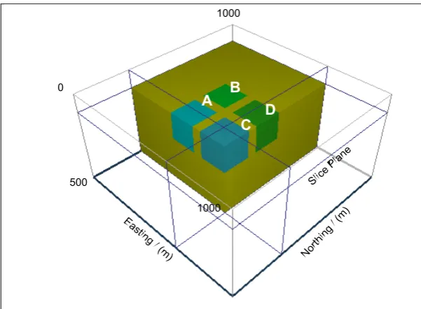
As Figure 1shows, a model consists of four geological targets (seen as rectangular boxes) embedded in the half-space. Density contrast and magnetization properties are assigned to the model (listed in Table 1). The anomaly is designed with different property values so that it can be recognized by petrophysical means. The ambient field has an inclination I= 45˚ and a declination D= 45˚. The observed response is modeled using gra v-ity and magnetic forward programs with 2.5% Gaussian noise.
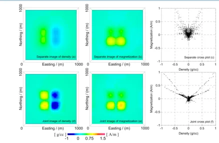
The recovered slices of density contrast and magnetization distribution horizontally located at depth = 200 m are shown in Figure 2. It is obvious that the separately imaged anomaly (top) reflects the basic feature of the rectangular boxes, but the resolution is low. Note that the interval between two adjacent boxes is blurred due to the smoothness hypothesis. A significant improvement in the jointly imaged density model is to distinguish anoma-lies with the same attributes. The boundary between two boxes with opposite attributes is also sharpened, thanks to the cooperation between the interactive structural constraints. The magnetization image has a similar appearance to the density image, and the image amplitude is enhanced when compared to the separate results, showing that the joint images have an enhanced focussing feature.
[image:3.595.155.456.358.579.2]The cross-plot of the two properties is a practical tool for demonstrating congruent relationships in the spatial scale (shown in Figure 2(c) and Figure 2(f)). Because of the smoothness constraints of the inversion scheme, the results tend to produce broad tails around the anomalies, which are displayed in the form of fuzzy cluster clouds (shown in Figure 2(c)). Fortunately, the divergence phenomenon is suppressed such that it is compressed close to the feature trends. This characteristic shows the potential for extracting additional information from the results and thus produces images that are both more detailed and more reliable.
Figure 1. Schematic of four geological units embedded in a uniform host medium.
Table 1. Rock physics of the subsurface medium.
Density contrast (g/cm3) Magnetization (A/m)
Half space 0.0 0.0
Rock A 1.0 1.0
Rock B 1.0 0.5
Rock C −1.0 1.0
Rock D −1.0 0.5
0
500
1000 1000
A B
[image:3.595.154.472.620.719.2]Figure 2. Images of density and magnetization distribution at horizontal slicing plane for depth = 200 m and cross-plots of property in spatial scale: (a) separate density image; (b) separate magnetization image; (c) density-magnetization cross-plot for the separate case; (d) joint density image; (e) joint magnetization image; (f) density-magnetization cross-plot for the joint case.
The joint inversion results show that lithological characterization can readily be conducted for any relation-ship that is more obvious in the cross-plot. In addition, a domain transform is used to amplify the difference be-tween geological targets, and also the contrast with the homogenous background. That is:
(
)
(
)
(
)
(
)
(
)
(
)
(
(
)
)
1 2
, , , , , , ;
, , , , ;
Im , ,
, , arctan .
Re , ,
c x y z m x y z im x y z r x y z c x y z
c x y z x y z
c x y z
θ
= +
=
=
(3)
where i is a complex unit; c is an artificial complex number composed of real part m1 and imaginary part 2
m ; r is the modulus of c; and θ is the azimuth angle of c on the complex plane. Figure 3 shows the radius- azimuth angle from which the anomaly can be identified by the vertical trends at different angles. The four geo-logical targets are recognizable from the bar-graph-like distribution. The low values homogeneously located close to the zero line are regarded as the host rock contaminated by noise. The spatial targets are recovered which is shown in Figure 3. All anomalous types have been divided successfully and their locations match the originals reasonably well when compared withFigure 1.
To sum up, the convergence of the relationship between two properties makes it possible to classify different types of subsurface medium based on the distinguishing feature line. The domain transform of the physical properties amplifies the differences between the geological targets, and make it easier to differentiate between anomalous bodies and host rock.
4. Application to Field Data
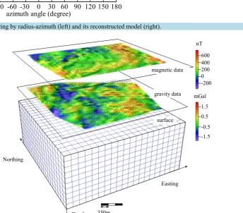
area measuring 7 × 8 km2 (Figure 4). The data was appropriately gridded to carry out 2-D low pass filtering in
[image:5.595.91.536.221.425.2]order to eliminate the negative influence of high-frequency noise. The study area is located in the effusive rock basin formed during faulting and magmatic activities in the late Yanshan. This district is mainly dominated by andesitic volcanic rock, volcanoclastics, tuff, syenite, etc. The orebody deposit occurs mainly within the tecton-ically crushed zone and fractured andesite.
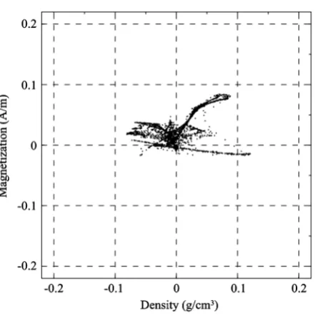
Figure 5 shows the cross-plot of joint inverted density and magnetization distribution. By incorporating struc-tural constraints, the results are consistent, as further shown by the distinct trends on the cross-plot. This reveals the potential for conducting advanced analysis using the proposed lithological characteristics technique. The ra-dius-azimuth plot, which is converted from the physical properties plane of Figure 5, is shown inFigure 6. The red rectangular boxes were marked manually in this presentation. In this case three types of rocks were generally
Figure 3. Anomaly filtering by radius-azimuth (left) and its reconstructed model (right).
Easting
350m Depth
Northing
surface gravity data magnetic data
600 400 200 0 -200
1.5 0.5 -0.5 -1.5 mGal
[image:5.595.96.542.230.686.2]nT
Figure 4. 3-D sketch map of disctreted subsurface materials and its observed gravity and magnetic field data.
0
500
1000 1000
A B C D
-180-150-120 -90 -60 -30 0 30 60 90 120 150 180 -0.5
0 0.5 1 1.5
azimuth angle (degree)
ra
di
us
[image:5.595.176.521.393.695.2]Figure 5. Cross plot of density and magnetization after joint inversion.
Figure 6. Anomaly filtering by radius-azimuth. The boxes in- dicate identified rock types.
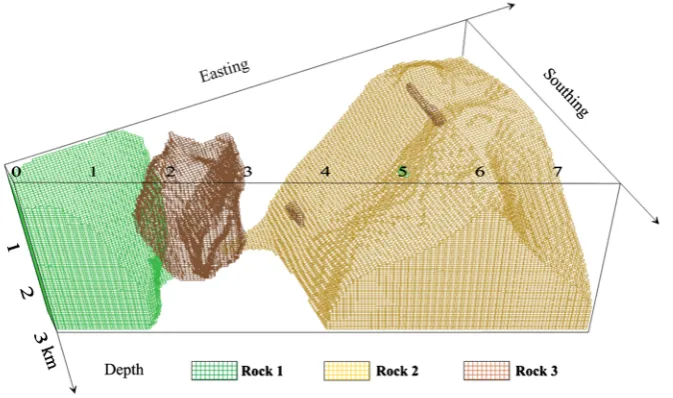
extracted from the whole subsurface, leading to the recovered lithology model presented in Figure 7. Rock 1 re-flects the physical trends near azimuth angle 0˚, which shows slight density and magnetization anomalies. Rock 2 delineates the high density and magnetization volume in the northeast of the study area. Rock 3 reveals nega-tive density contrast and medium magnetization anomalies. Preliminary geological inferences and rock sample analyses suggested that the volcanic rocks stratum rises in the northeastern region, showing both high density contrast and magnetism, and the crater area is located beneath sedimentary overburden in the central northwes-tern region, showing low density contrast and high magnetism. All these lithological characteristic interpreta-tions match the geological inferences.
5. Conclusion
Figure 7. Lithological characterization analysis extracted from joint imaging results.
Acknowledgements
This work was funded by National Natural Science Foundation of China, Beijing Higher Education Young Elite Teacher Project (YETP0650), The National High Technology Research and Development program (“863” Pro-gram) of China (No. 2013AA063901-4 and 2013AA063905-4), R&D of Key Instruments and Technologies for Deep Resources Prospecting (The National R&D Projects for Key Scientific Instruments) (No. ZDYZ2012-1- 02-04), Constrained multi-parameter inversion of geophysical technology and software systems (No. 2014AA06A613), and The Fundamental Research Funds for the Central Universities.
References
[1] Yan, J.Y., Lü, Q.T., Chen, X.B., Qi. G., Liu, Y., Guo, D. and Chen, Y.J. (2014) 3D Lithologic Mapping Test Based on 3D Inversion of Gravity and Magnetic Data: A Case Study in Lu-Zong Ore Concentration District, Anhui Province.
Acta Petrologica Sinica, 30, 1041-1053.
[2] Kanasewich, E.R. and Agarwal, P.G. (1970) Analysis of Combined Gravity and Magnetic Fields in Wave Number Domain. Journal of Geophysical Research, 75, 5702-5712. http://dx.doi.org/10.1029/JB075i029p05702
[3] Price, A. and Dransfield, M. (1995) Litholgical Mapping by Correlation of the Magnetic and Gravity Data from Corsai W.A. Exploration Geophysics, 25, 179-188. http://dx.doi.org/10.1071/EG994179
[4] Lane, R. and Guillen, A. (2005) Geologically-Inspired Constraints for a Potential Field Litho-Inversion Scheme. In: Frits, B. and Graeme, B.C., Eds., Proceedings of IAMG: GIS and Spatial Analysis. Annual Conference of the Interna-tional Association for Mathematical Geology, Toronto. International Association for Mathematical Geology, Toronto, 181-186.
[5] Williams, N. C. and Dipple, G. (2007) Mapping Subsurface Alteration Using Gravity and Magnetic Inversion Models. In: Milkereit, B., Ed., Proceedings of the Fifth Decennial International Conference on Mineral Exploration. Fifth De-cennial International Conference on Mineral Exploration, Toronto. Prospectors and Developers Association of Canada, Toronto, 461-472.
[6] Kowalczyk, P., Oldenburg, D.W., Phillips, N., Nguyen, T.H. and Thomson, V. (2010) Acquisition and Analysis of the 2007-2009 Geoscience BC Airborne Data. In: Lane, R.J., Ed., Expanded Abstracts of ASEGPESA Airborne Gravity Workshop. ASEG-PESA Airborne Gravity Workshop, Canberra. Geoscience Australia, Canberra, 115-124.
[7] Infante, V., Gallardo, L.A., Montalvo-Arrieta, J.C. and de León, I.N. (2010) Lithological Classification Assisted by the Joint Inversion of Electrical and Seismic Data at a Control Site in Northeast Mexico. Journal of Applied Geophysics,
70, 93-102. http://dx.doi.org/10.1016/j.jappgeo.2009.11.003
[8] Gallardo, L.A. and Meju, M.A. (2003) Characterization of Heterogeneous Near-Surface Materials by Joint 2D Inver-sion of dc Resistivity and Seismic Data. Geophysical Research Letters,30, 1658.
[9] Gallardo, L.A. and Meju, M.A. (2004) Joint Two-Dimensional DC Resistivity and Seismic Travel Time Inversion with Cross-Gradients Constraints. Journal of Geophysical Research: Solid Earth, 109, B03311.
http://dx.doi.org/10.1029/2003JB002716
[10] Li, Y. and Oldenburg, D.W. (1996) 3-D Inversion of Magnetic Data. Geophysics, 61, 394-408.
http://dx.doi.org/10.1190/1.1443968
[11] Fregoso, E., Gallardo, L.A. (2009) Cross-Gradients Joint 3D Inversion with Applications to Gravity and Magnetic Data.