New Physics Models in the Diphoton Final State at CMS

(1)

New Physics Models in the Diphoton Final State at CMS

Thesis by

Ann Miao Wang

In Partial Fulfillment of the Requirements

for the Degree of

Bachelor of Science

California Institute of Technology

Pasadena, California

2015

(2)

c

2015

Ann Miao Wang

(3)

Acknowledgments

First, I want to express my gratitude to Professor Maria Spiropulu for being the most inspirational

leader, mentor, and scientist I could have ever hoped to work for. My deep interest in experimental

high energy physics is a result of her passion and tireless enthusiasm for the subject.

I would also like to express my deep appreciation for Professor Harvey Newman for being a

wonderful teacher and listener. His diligence and love for physics have painted him as a true role

model in my life.

I am extremely grateful to Javier Duarte for always answering my questions and meeting with

me for a countless number of hours over the past three years. His kindness and patience have made

an indescribable impact on my research experience.

I would also like to Cristian Pe˜na, Dustin Anderson, Alex Mott, and Maurizio Pierini, as well as

the entire Caltech CMS group, for their invaluable guidance throughout this thesis.

These past four years at Caltech have truly been life-changing in completely surprising ways.

One was my unexpected passion for studying physics, which I could not have anticipated. I owe that

to the professors and students at this remarkable institution, especially Professor Steven Frautschi

for instilling his enthusiasm in me through Ph 1 recitations. Without his extraordinary teaching, I

would never have switched my major to physics.

Finally, I would like to express my gratitude to my parents and my sister for their love and

(4)

List of Figures

2.1 A cartoon of a disquark production scenario. . . 2

3.1 Comparisons of the razor variables formed with PF objects versus calorimeter objects. 6

3.2 Comparisons of theE/T distributions formed with PF objects versus calorimeter objects. 6

3.3 Comparisons of theE/T andR2distributions formed with PF objects versus calorimeter

objects, vetoing all events that have muons withpT >30 GeV. . . 6

3.4 Schematic of the H→b¯btrigger flow path. The numbers in parentheses correspond to the more detailed list described in the text. . . 9

4.1 The contour lines forM∆= 450 GeV, whereM∆=m

2 ˜

b−m

2 ˜

χ

m˜b , with±50 GeV as indicated by the dashed lines. . . 14

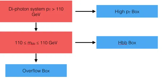
4.2 A schematic for how events are placed into the three boxes. The red rectangles are the

two requirements, and the blue rectangles represent the boxes. . . 15

4.3 Z-axis scale units are such that the total number of events is normalized to 1. m˜_b= 600

GeV,m_χ_˜0

1 = 300 GeV model. (a)R

2 _versus_M

R for the 50% (to ˜χ02) working model. (b)R2_versus_M

Rfor the 100% (to ˜χ02) working model. (c)R2versusMRfor the 90%

(to ˜χ0

2) working model. (d)R2 versusMR for the 10% (to ˜χ02) working model. . . 17 4.4 Z-axis scale units are such that the total number of events is normalized to 1. m˜_b =

600 GeV, mχ˜0

1 = 300 GeV model. (a) R

2 _versus _E_/

T , for the 50% (to ˜χ02) working model. (b)R2versusE/T , for the 100% (to ˜χ02) working model. (c)R

2_versus_E_/

T , for

the 90% (to ˜χ02) working model. (d)R2 versusE/T , for the 10% (to ˜χ02) working model. 18

4.5 Z-axis scale units are such that the total number of events is normalized to 1. m˜_b= 600

GeV,m_χ_˜0

1 = 300 GeV model. (a) MR versus E/T for the 50% (to ˜χ

0

2) working model.

(b)MR versusE/T , for the 100% (to ˜χ02) working model. (c) MR versus E/T , for the

90% (to ˜χ0

2) working model. (d) MR versusE/T , for the 10% (to ˜χ02) working model. . 19 4.6 Characterization of them˜_b= 550 GeV,mχ˜0

1 = 300 GeV model with 90% to ˜χ

0

2. Z-scale

units are such that the total number of events is normalized to 1. (a) R2 _versus_M

R.

(b) R2 _versus _E_/

T . (c) MR versus E/T . (d) Number of PF jets, clustered with the

(7)

4.7 Characterization of them˜_b = 450 GeV,m_χ_˜0

0 2.

Z-scale units are such that the total number of events is normalized to 1. (a)R2 _versus

MR. (b)R2 versus E/T . (c) MR versus E/T . (d) Number of PF jets, clustered with

the anti-kT algorithm with ∆R = 0.5. . . 22

4.8 Characterization of them˜_b = 530 GeV,mχ˜0

0 2.

Z-scale units are such that the total number of events is normalized to 1. (a)R2 versus

4.9 Razor variable distributions for the various mass splitting with fixed ˜χ0

1mass. (a)MR

1D distributions. (b)R2 _{1D distributions.} _{. . . .} ₂₄

4.10 Kinematic distributions for the various mass splitting with fixed ˜χ0

1 mass. (a)E/T 1D

distributions. (b) Leading jetpT 1D distributions (excluding H → b¯bjets). . . 24

4.11 The decay spectrum for them˜_b= 450 GeV model. . . 25

0 2.

4.14 Razor variable distributions for the various mass splitting with fixed ˜b mass. (a) MR

1D distributions. (b)R2 _{1D distributions.} _{. . . .} ₂₈

4.15 Kinematic distributions for the various mass splitting with fixed ˜b mass. (a) E/T 1D

distributions. (b) Leading jetpT 1D distributions (excluding H → b¯bjets). . . 28

4.16 χ˜0₁kinematic distributions for the various mass splitting with fixed ˜bmass. (a) Leading

˜

χ0₁ pT 1D distributions. (b) ∆Φ between the two ˜χ01 particles. . . 29

4.17 Bottom squark kinematic distributions for the various mass splitting with fixed ˜bmass.

(a) Leading ˜b pT 1D distributions. (b) ∆Φ between the two bottom squarks particles. 29

0 2.

(8)

0 2.

4.20 The decay spectrum for them˜_b= 470 GeV model. . . 32

4.21 Razor variable distributions for the various ˜b models with fixed M∆. (a) MR 1D

distributions. (b)R2 1D distributions. . . 33

4.22 Kinematic distributions for the various ˜b models with fixedM∆. (a) Leading jet pT

1D distributions (excluding H → b¯b jets). (b) Subeading jet pT 1D distributions

(excluding H→ b¯b jets). (c) Leading ˜χ0

1 pT 1D distributions. (d) Subeading ˜χ01 pT

1D distributions. . . 33

4.23 Kinematic distributions for the various ˜bmodels with fixedM∆. (a) Leading ˜b pT 1D

distributions. (b) Subleading ˜b pT 1D distributions. (c) ∆Φ between the two bottom

squarks particles. (d) ∆Φ between the two ˜χ0

1 particles. . . 34

4.24 Event populations of the CLT2015-AW1 Model at √s = 8 TeV in each of the boxes, with the total amount of events passing the selection scaled to 100. (a) High pT box

(b) Hbb box (c) Overflow box. . . 35

4.25 Event populations of the SM Higgs production background at√s= 8 TeV in each of the boxes, with the total amount of events passing the selection scaled to 100. (a) High

(9)

Chapter 1

Introduction

With the discovery of the Higgs boson as the final particle necessary to complete the standard model

(SM) picture [1, 2], the field of particle physics is looking towards the search for new physics outside

of the SM. One problem with the SM is that it does not include a viable particle candidate for

dark matter [3]. At the Large Hadron Collider (LHC) in Geneva, Switzerland, scientists are looking

for beyond-the-standard-model (BSM) events resulting from proton-proton collisions. One possible

BSM physics scenario is weak-scale supersymmetry (SUSY) which provides a particle candidate for

dark matter and solves the heirarchy problem [4].

A major difficulty in any search for new physics is to characterize what the signatures of the

BSM physics would look like at the detector level. In the search for these events, there are many

components of a physical experiment that must be studied and tuned. This thesis addresses two

of the most important components: (1) trigger studies and (2) model kinematics. The overarching

theme of this thesis is the use of the newly discovered Higgs particle as a probe for searching for

BSM physics. The first half of the thesis focuses on studies related to the Compact Muon Solenoid

(CMS) detector, while the second half of the thesis is more broadly applicable to other experiments.

Chapter 2 gives a short overview of the razor variables, which have been used to distinguish SUSY

from SM background, producing strong limits on SUSY models [5]. The thesis will then employ these

razor variables in the design of the custom hardware and software algorithms for deciding whether

to record a collision event, and will investigate the distribution of these variables for certain SUSY

simplified models.

Chapter 3 focuses on trigger design for BSM searches. It first tackles the study of the

software-level trigger (known as the High Level Trigger) paths using the razor variables. Then, it includes

a proposal of a new trigger path targeting BSM events that include a Higgs boson decaying to a

b¯b pair in the final state. Chapter 4 is motivated by a previous search for supersymmetry with a

Higgs decaying to two photons [6]. It discusses the kinematics of Higgs-aware BSM models, with

particular focus on bottom squark production. This thesis attempts to fully characterize the range

(10)

Chapter 2

The Razor Variables

The razor variables,MRandR2, are variables that are useful in searches for supersymmetry (SUSY).

They have been successfully employed in previous searches with the CMS Collaboration to produce

strong limits on SUSY parameter space [7]. These variables are employed to help distinguish SUSY

signal events from the Standard Model (SM) background.

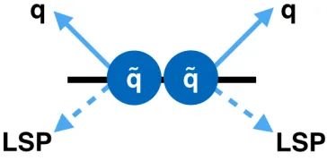
Figure 2.1: A cartoon of a disquark production scenario.

If we consider the scenario where two squarks (supersymmetric partners of quarks) each decay

to a quark and a stable, weakly interacting lightest supersymmetric particle (LSP), the missing

energy carried away by the LSP makes it difficult to reconstruct the kinematic attributes of all the

particles in the decay. Thus, it is a challenge to identify this as a SUSY decay. For an all-hadronic

analysis, we form the two razor variablesMR, R2as follows: first, we cluster the hadronic jets into

two hemispheres using an algorithm in which we minimize the sum in quadrature of the invariant

masses of the two hemispheres. These jets often have some baseline thresholds for certain kinematic

events, such as transverse momentum (pT) or pseudorapidity (η). Then, we defineMR as

MR= q

(|pj1_|₊_|_pj2_|₎2₋₍_pj1

z +pjz2)2,

wherepjiis the momentum of the ith hemisphere. R is defined as

(11)

where

M_TR=

s / ET(p

j1

T +p j2

T)−E~/T ·(~p j1

T +~p j2

T )

2 ,

andE/T is the missing transverse energy of the event.

MRis contains information about the characteristic SUSY mass scales. It is an estimator, in the

case of the squark, forM∆, which we define to be

M∆=

m2_q_˜−m2_χ_˜ m˜q

.

m˜q is the mass of the squark, and mχ˜ is the mass of the LSP. Experimentally, MR peaks higher

for SUSY events. R2 contains information about the missing energy in the event and helps reduce

QCD backgrounds [7]. Because of these advantages, the razor variables have been implemented

successfully for new physics searches.

(12)

Chapter 3

CMS Trigger Studies

3.1 The CMS Detector and the Trigger System

The CMS detector is a general purpose detector at the LHC with various sub-detector components.

It includes a lead-tungstate-crystal electromagnetic calorimeter (ECAL), a hadronic calorimeter

(HCAL), a silicon tracker, and a muon drift tube system, cathode strip chambers, and resistive

plate chambers [8]. The next run of the LHC, scheduled to begin in 2015, requires both software

and hardware improvements due to higher energies (13 and 14 TeV) of the proton-proton collisions

as well as increased underlying event activity (known as pileup) [9]. The events detected by CMS

are too large in number to record all of the data, so a trigger system is required to decide which

collision events to record.

This trigger system is composed of two levels; the system results in data reduction from the LHC

collision rate of 15 MHz down to a rate of 400 Hz for Run 1 (and 1 kHz for Run 2). The two levels

are the hardware-based Level-1 (L1) system and the software-based High Level Trigger (HLT). In

order to minimize CPU time, particle and event kinematics are only partially reconstructed since

triggering is conducted in real-time [10, 11].

The L1 system has three main components: global, muon, and calorimeter. The L1 calorimeter

system is based on a set of trigger towers, which are made up of 4×4 regions. These regions are each 20◦ _in_φ_{(azimuthal angle), and are also sectioned by}_η _{(pseudorapidity). Jets, which are the result}

of quark and gluon production in the detector, are calorimeter objects at the L1 level.

One or more L1 filters can feed into an HLT filter. For the HLT system, muons are reconstructed

using isolation algorithms and track fitting, which involves matching inner tracker tracks with outer

muon spectrometer tracks. There are two possible collections of jets andE/T at the HLT: calorimeter

collections and Particle Flow (PF) collections. Calorimeter objets are crude objects reconstructed

from energy deposits in the calorimeters, while PF objects are more sophisticated and rely on the

PF algorithm [12]. The PF algorithm takes information from the multiple sub-detectors to produce

(13)

particle information. These particles are then clustered using the anti-kT jet clustering algorithm

to reconstruct the jets [13, 14].

The selected kinematic thresholds for both the L1 and HLT must be thoroughly tested to (1)

ensure sufficient data reduction and to (2) maintain the efficiency of keeping events which are

interesting for our physics analyses. We will focus on the HLT in the following section.

3.2 Razor High Level Triggers

A set of trigger options involving razor variables were implemented for the LHC Run I. Due to higher

energies, increased pileup, and shorter bunch spacing, these triggers need to be modified for Run II.

In addition, PF objects are now available at the HLT, so the option of using PF objects instead of

calorimeter objects must be discussed.

Although PF objects have been shown to have a much improved accuracy [15], they are more

costly in CPU time at the HLT. As a result, one tactic of using PF objects but still minimizing CPU

time is to reduce the number of events that the PF algorithm acts on by imposing loose thresholds

on calorimeter-level objects.

One important detail before implementing this tactic is to study the correlation of PF objects

to calorimeter objects.

3.2.1 Calorimeter Objects versus PF Objects Investigation

Because calorimeter objects and PF objects are constructed differently, we conducted a study of PF

versus calorimeter variables. We conducted this study with a sample oft¯t+jets, common background

to many SUSY signals. This particular sample forcest¯tto decay leptonically, and details are in Table

A.3. The main variables we were concerned with were the razor variables since the HLT triggers

include cutoffs based on these variables. Thus, we studied the razor variables constructed with PF

objects versus calorimeter objects. Examining Figure 3.1, the R2 _{correspondence is much worse}

than theMR correspondence. In addition to using the jet object information, theR2 variables are

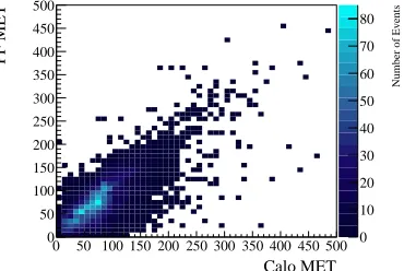
constructed using the E/T information. We then investigated the correspondence between PF and

caloE/T, shown in Figure 3.2.

When the HLT E/T is calculated using energy deposit information from the hadronic and

elec-tromagnetic calorimeters [10], the information from the muon chambers is excluded. As a result, we

suspected that the muon energies were not correctly incorporated into the calorimeter-levelE/T. To

investigate this, we replotted the distributions with the additional requirement that muons withpT >

30 GeV be vetoed. A remarkable improvement of the correspondence between PF and calorimeter

/

(14)

Number of Events 0 20 40 60 80 100 R Calo M

0 500 1000 1500 2000 2500

R PF M 0 500 1000 1500 2000 2500 (a)

Number of Events

0 20 40 60 80 100 120 140 2 Calo R

0 0.1 0.2 0.3 0.4 0.5 0.6 0.7 0.8

2 PF R 0 0.1 0.2 0.3 0.4 0.5 0.6 0.7 0.8 (b)

Figure 3.1: Comparisons of the razor variables formed with PF objects versus calorimeter objects.

Number of Events

0 10 20 30 40 50 60 70 80 Calo MET

0 50 100 150 200 250 300 350 400 450 500

PF MET 0 50 100 150 200 250 300 350 400 450 500

Figure 3.2: Comparisons of theE/T distributions formed with PF objects versus calorimeter objects.

Number of Events

0 10 20 30 40 50 60 Calo MET

0 50 100 150 200 250 300 350 400 450 500

PF MET 0 50 100 150 200 250 300 350 400 450 500 (a)

Number of Events

0 10 20 30 40 50 60 70 80 90 2 Calo R

0 0.1 0.2 0.3 0.4 0.5 0.6 0.7 0.8

2 PF R 0 0.1 0.2 0.3 0.4 0.5 0.6 0.7 0.8 (b)

Figure 3.3: Comparisons of theE/T andR2distributions formed with PF objects versus calorimeter

objects, vetoing all events that have muons withpT >30 GeV.

Following these studies, recommendations were made for muon information to be incorporated

into the calorimeter level razor variables. Muon information was then added to the hemisphere

(15)

3.2.2 Trigger Flow Path

For a trigger involving the razor variables, the trigger path is as follows:

1. Input from the Level 1 CMS Hardware Trigger. For these triggers, a combination of all hadronic

triggers available were used.

2. Algorithms to create calorimeter objects, which use information from the calorimeter [13].

3. Thresholds implemented on the calorimeter jet kinematic properties.

4. Thresholds implemented on the razor variables constructed from calorimeter objects.

5. Algorithms to create Particle Flow (PF) objects, which use an increased amount of available

information from CMS [13].

6. Thresholds implemented on the PF jet kinematic properties.

7. Thresholds implemented on the razor variables.

3.2.3 Rates of Trigger Menu

Various triggers were investigated to optimize the thresholds at the PF level and the calorimeter

level. To calculate these rates, the triggers were evaluated within the CMS HLT software framework

[16] over a weighted average of a set of QCD Monte Carlo samples (see Table A.1) with various jetpT

bins from 30 to 100 GeV, with 40 pile-up (pp collisions per bunch) and bunch-crossings happening

every 25 ns. These samples essentially consisted of jets and pileup events.

The triggers are in part named according to CMS convention. A short code follows:

1. Rsq0pX indicatesR2_>_0.X.

2. MRX indicates MR>X.

3. RsqMRX indicates (R2−0.25)∗(MR−300)>X. These offsets of 0.25, 300 approximate the

R2_∗_M

R iso-probability contours observed in the CMS 8 TeV dataset [17].

4. NoRazorCaloCut indicates all calorimeter-level filters on the razor variables are removed.

Trigger Name Rate (Hz)

HLT RsqMR300 Rsq0p09 MR200 12.471±1.244

HLT RsqMR300 Rsq0p09 MR200 Muon 12.472±1.244

(16)

HLT RsqMR300 Rsq0p09 MR200 Muon NoRazorCaloCut 12.967±1.249

HLT RsqMR300 Rsq0p09 MR200 Muon CaloRsq0p0196 11.188±1.145

Table 3.2: Table of the razor triggers discussed, where the rate is calculated for an instantaneous lu-minosity of 1.4e34 cm−2_s−1_{. These have a calorimeter-level filter of hltRsqMR240RsqXMR100Calo,} where X = 0.0196 for the second trigger and X = 0.0289 for the third trigger. All triggers have the muon sequence enabled.

Table 3.3: Table of the razor triggers discussed, where the rate is calculated for an instantaneous lu-minosity of 1.4e34 cm−2_s−1_{. These have a calorimeter-level filter of hltRsqMR260RsqXMR100Calo,} where X = 0.04 for the first trigger and X = 0.0576 for the second trigger. All triggers have the muon sequence enabled.

We first investigated the addition of the muon sequence mentioned in the previous section. We

see that the rate increases marginally in Table 3.1. Therefore, adding the muon sequence to the

calorimeter razor variables does not noticeably increase the rate, but would have a beneficial effect

on accuracy for backgrounds and signals with a lot of muons, i.e. t¯t+jets.

We then investigate the effect of the calorimeter-level razor variable thresholds on rate. Ideally,

an increase in calorimeter-level razor variable thresholds would have a minimal effect on the rate

when the thresholds are lower than the following PF thresholds. The PF thresholds implemented

without any calorimeter-level thresholds on the razor variables are given in line 1 of Table 3.2.

As we increase the calorimeter-level razor thresholds, we see the rate slowly decrease to ≈ 10 Hz, which is around the rate that we desire. Note that for Table 3.3, we also raise the R2_×_M

R

threshold in order to match the increase in R2_{. This illustrates the fact that there is still a small}

mismatch between calorimeter objects and PF objects.

3.3 H

→

b

¯

b

HLT Trigger

3.4 Motivation

Investigation of an H→b¯b trigger has been conducted for possible addition to the Run II trigger menu. This is motivated by the use of Higgs detection as a tool for finding new physics, which will

be further elaborated on in Chapter 3. Since H→b¯bis the dominant decay mode (branching ratio 57.8%) for a 125 GeV Higgs [18], this trigger is ideal for capturing the maximum amount of events.

However, the high SM cross section for bottom production at the LHC poses a problem for the rate

of events passing this trigger [19]. As a result, many kinematic thresholds have to be combined in

(17)

3.5 b-tagging

Bottom quarks, or b quarks, are found in many supersymmetric processes [20]. CMS has several

algorithms for b quark identification, or b-tagging. For our study, we will use the Combined

Sec-ondary Vertex (CSV) algorithm. This algorithm assigns a value to each jet which indicates the

probability of misidentification. There are three working points for this algorithm: loose, medium,

and tight, which correspond to ≈10%, ≈1%, and ≈0.1% probabilities for an average jet pT of 60

GeV [21]. These algorithms rely on tracks as well as secondary vertices, which can indicate the

lifetime of quark before decay. This exploits the fact that the b quark has a relatively long lifetime,

≈1 picosecond [22]. CSV loose, medium, and tight points also result in varying b-tag efficiencies.

The loose point corresponds to≈80-90% efficiency, medium to≈60-70% efficiency, and tight to≈

50% efficiency [21].

3.6 Trigger Flow Path

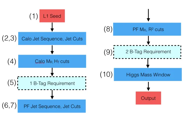
Figure 3.4: Schematic of the H→b¯b trigger flow path. The numbers in parentheses correspond to the more detailed list described in the text.

The trigger flow path is as follows (Figure 3.4):

1. Input from the Level 1 CMS Hardware Trigger. For these triggers, a combination of all hadronic

triggers available were used.

2. Algorithms to create calorimeter objects, which use information from the calorimeter [13].

(18)

4. Thresholds implemented on encompassing variables, such as the razor variables orHT, which

is a sum of transverse hadronic energies.

5. At least one b-tagged jet with a specified CSV threshold (see Section 3.5).

6. Algorithms to create Particle Flow (PF) objects, which use an increased amount of available

information from CMS [13].

7. Thresholds implemented on the PF jet kinematic properties.

8. Thresholds implemented on the razor variables.

9. At least two b-tagged jets with specified CSV threshold (see Section 3.5).

10. Higgs mass window filter applied to any two b-tagged jets that pass the specified CSV

require-ments in the previous step.

3.7 Rates of H

→

b

¯

b

Trigger

The naming convention carries from Section 3.2.3. A few more abbreviations are as follows:

1. BTagXCSV0YCSV0Z indicates that there are X b-tags required, with a Combined Secondary

Vertex (CSV) cutoff of 0.Y and 0.Z for two PF jets. For calorimeter jets, there is a CSV cutoff

of 0.Y - 0.1 required for one jet. See Section 3.5 for further information on b-tagging.

2. DiJetX indicates that we require two PF jets with pT >X GeV, and for calorimeter jets we

require the leading jet to have pT >X - 10 GeV and the subleading jet to have pT >X - 20

GeV.

3. TriJetX indicates that we require three PF jets withpT >X GeV.

4. MqqMinXMaxY indicates that we require that there be two PF b-jets (with the b-tagging

CSV requirements from (1)) that have a invariant mass between X and Y GeV.

5. HTX indicatesHT >X GeV.

HLT BTag2CSV05CSV02 DiJet80 Rsq0p01 MR200 MqqMin70Max190 121.770±7.015

HLT BTag2CSV05CSV02 DiJet80 HT200 Rsq0p01 MR300 MqqMin70Max190 93.946±5.791

HLT BTag2CSV05CSV02 DiJet80 CaloMR200 Rsq0p01 MR300 MqqMin70Max190 93.384±5.774

HLT BTag2CSV05CSV02 DiJet80 TriJet40 CaloMR200 Rsq0p0196 MR300 MqqMin70Max190 61.056±5.333

HLT BTag2CSV07CSV04 DiJet80 CaloMR200 Rsq0p01 MR300 MqqMin70Max190 37.483±3.807

(19)

3.7.1 Addition of new HCAL local reconstruction method and ECAL

Multifit

An update of the calorimeter local reconstruction methods to handle out-of-time pile-up, which is

pile-up from adjacent bunch-crossing, was released [23]. This improved energy reconstruction in the

hadronic calorimeter endcap and barrel, relies on fitting measured pulses with parameterizations

derived from test pulses, then subtracting the out-of-time pileup contribution from the energy

mea-surement. This technique results in better resolution and measurement [24]. A similar update was

released for the electromagnetic calorimeter to reduce out-of-time pileup by simulating and fitting

the pulse shape from an average of pulses from samples shifted from each other in bunch-crossings

[25]. We applied this technique to two of our proposed triggers and measured their rates.

Table 3.5: Table of theH →b¯btriggers discussed, where the rate is calculated for an instantaneous luminosity of 1.4e34 cm−2s−1.

3.7.2 Discussion

The rates are shown in Table 3.4. We see that the tightening of the CSV thresholds sharply reduces

the rate. The addition of the razor variable orHT cut is also effective at reducing the rate and is

low enough to keep high signal events. We refrain from a highR2threshold in an effort to select for

different events from the regular razor triggers. We also keep a relatively large Higgs mass window

since the main goal of this trigger is to keep events that include a Higgs.

The new ECAL and HCAL methods do not reduce the rates significantly (Table 3.5), but should

(20)

Chapter 4

Investigation of Higgs-Aware

Decay Models

4.1 The Higgs decay as a tool for new physics searches

Armed with the discovery of the Higgs Boson, we are able to employ the Higgs as a tool for future

physics studies. We can study its mass and other properties, which have implications for the possible

existence of beyond-the-standard-model (BSM) phenomena including SUSY and dark matter. We

can also use the Higgs boson as a probe for searching for new physics. For example, the Higgs

invisible decay channel has been ideal for BSM studies since the branching fraction of the purely SM

decay,h→ZZ∗→4ν is small [26]. There have already been studies exploiting this channel [27]. Similarly, we can employ the Higgs to look for SUSY by targeting decays that specifically produce

a Higgs, such as those that include a next-to-lightest neutralino decaying to a Higgs and a lightest

neutralino, χ0

2 → hχ01 [28]. The decay of the Higgs to two photons has been observed as a clean, sharp signal [29] and is an ideal decay channel to target. A previous search for supersymmetry with

this decay channel motivates this thesis work [6], but we will examine different SUSY models from

the search.

4.2 Motivation

Many standard SUSY searches rely on missing transverse energy (E/T) in order to separate signal

from Standard Model background. E/T is calculated from energy deposits in the subdetectors [30].

As a result, strong limits have been placed for SUSY models with largeE/T [31]. These standard

searches look for models with signal events at R2 _{values of greater than 0.2 - 0.3 [28]. Instead, we}

would like to investigate models with lowerE/T and lower R2, which may have eluded LHC bounds

but are good candidates for Run II.

(21)

background from our analysis. We can then study models with lessE/T and look in areas of the SUSY

phase space that have not been extensively studied. We will focus on bottom squark production

decaying to Higgses, rather than top squark production. In general, since top quarks decay to a W

boson and a bottom quark, top squark models have more complicated topology with higherE/T due

to the W bosons decaying to neutrinos.

Our goal is to study a viable model for a LHC Run II analysis. In order to achieve this, this

thesis will explore the different kinematic parameters in bottom squark production and decay. In

particular, we desire models which have lowE/T, lowR2, and MR values clustered from 400 to 500

GeV. HigherMR values have a higher probability of already being excluded, and at too low ofMR

we lose events from the trigger thresholds.

We can consider a model where we have a bino-like next-to-lightest supersymmetric particle

(NLSP) which would decay predominantly to a Higgs boson and a weakly coupled LSP [32]. The

next-to-lightest neutralino can be considered the NLSP, and the lightest neutralino is the LSP. For

the dominant mode of bottom squark production, the final state particles will be two bottom quarks

and two Higgs bosons.

CMS SUSY searches are interpreted in the context of simplified models [20]. A simplified model

consists of only relevant particles, specifying the particle production and subsequent decay. It is

defined by the model parameters that would influence how an event would look in the detector.

For example, the T2qq model described in [20] is a simplified model that focuses on pair-produced

squarks decaying to two quarks and two LSPs, where the free parameters are masses of the squark

and the LSP. We will use this interpretation for our studies.

4.3 Bottom squark production model

We investigated a bottom squark production model, where the bottom squark has two possible

decays channels: ˜b→bχ˜0₂→bHχ˜0₁, and ˜b→bχ˜0₁.

The bottom squark particle can be produced through several mechanisms, see Section A.2. The

dominant production modes result in pair production.

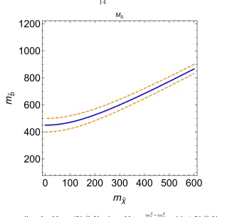
We wanted to obtainMRpeak values from 400-500 GeV for these events, and we needed to comply

with current exclusion limits [33]. Note that these exclusion limits assume a decay of ˜b →bχ˜0 1. If

we examine Fig. 4.1, we see that the contour lines forM∆= 450±50 GeV become approximately linear at above ˜χ0

1≈ 200-250 GeV. Referring to the limits in [33], we see thatm˜b = 600 GeV and

mχ˜0

1 = 300 GeV is a good starting point. For all of the follow studies, the mχ˜02 is set at mχ˜01 +

130 GeV to minimize the E/T carried away by the lightest neutralino. After choosing appropriate

mass points, several working points of the branching ratios for the two decay channels of the ˜bwere

(22)

0 100 200 300 400 500 600

200

400

600

800 1000

1200

m

χ˜

m

b

˜

MΔ

Figure 4.1: The contour lines forM∆= 450 GeV, whereM∆=

m2 ˜

b−m

2 ˜

χ

m˜b

, with±50 GeV as indicated by the dashed lines.

Events were produced at 8 TeV center-of-mass energy using PYTHIA 8.1 [34, 35] interfaced with

SUSY Les Houches Accord (SLHA) files [36] and the BSMatLHC package [37]. They were filtered

using a selection process described in Section 4.4. The Higgs boson was forced to decay to two

photons.

4.4 Selection

After events were produced, several requirements were implemented to filter out the events. This

selection was loosely modeled after the aforementioned Higgs to diphoton supersymmetry search [6]

to reduce potential background, with modifications specific to a generator-level study.

1. The event must have a pair of photons that has a diphoton mass of >100 GeV. One of these

photons should have pT >40 GeV, and the other should have pT >25 GeV.

2. Then, if two pairs of photons that satisfy (1) are found, then one of them is randomly set aside

to later be counted as an alternate channel for Higgs decay besides two photons. This is done

to retain the maximum amount of events generated by PYTHIA.

(23)

4. The event must have at least one jet with pT >30 GeV and |η|<3.0, and have a ∆R >0.5

with respect to the either of the pair of photons selected. These jets are produced using the

PF algorithm, clustered with an anti-kT algorithm using ∆R = 0.5 [15, 14, 38].

5. We only keep jets withpT >30 GeV and|η|<3.0.

4.5 Box definitions

Figure 4.2: A schematic for how events are placed into the three boxes. The red rectangles are the two requirements, and the blue rectangles represent the boxes.

After selection, the events were further categorized into boxes for further discrimination of

poten-tial signal from background. These boxes are all restricted toMR∈[150,3000] GeV andR2∈[0,1].

The boxes are again motivated by the Higgs to diphoton supersymmetry search and are as follows:

1. High pT Box requirespT of the di-photon system to be>110 GeV.

2. Hbb Box requires 110 ≤ mbb ≤ 140 GeV, with mbb being the invariant mass of any two

b-tagged jets.

3. Overflow Box

The events are grouped into the boxes in a hierarchal system. So, if an event passes the requirements

for box 1, then it is grouped into box 1. If it fails and passes the requirements for box 2, then it

goes in box 2. Else, it goes into the Overflow Box (see Figure 4.2). These boxes are constructed to

characterize a potential SUSY signal from background events. The HighpT box selects for boosted

Higgs bosons (with high momentum), while the Hbb box allows us to select for diHiggs production.

For the Hbb box, we assume that the second Higgs produced would decay to two b quarks because

of the high branching ratio [18].

(24)

photon pairs is randomly set aside to be counted as an alternate channel. We apply a 57.8% chance

that this pair should be counted as a H →b¯b decay channel to simulate the branching ratio [18]. Then, with every b-jet in the event, we emulate the b-tagging efficiency by randomly tagging 60%

of generator level b-jets. This approximately corresponds to the efficiency of a CSV medium b-tag

requirement (see Section 3.5). The reason this artificial handling of bottom quarks is necessary so

we do not overestimate the number of events that would fall in the Hbb box. These box definitions

are important for future inclusive analyses and will be used in the later statistical study in Section

4.11.

4.6 Branching Ratio to

χ

˜

0₂

Study

m

˜_b

m

χ˜0

2

m

χ˜01

BR (to ˜

χ

0 2

)

600 GeV

430 GeV

300 GeV

10%

600 GeV

430 GeV

300 GeV

50%

600 GeV

430 GeV

300 GeV

90%

600 GeV

430 GeV

300 GeV

100%

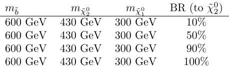
Table 4.1: Table of the models investigated in the branching ratio study, with their associated values ofM∆andMsplit.

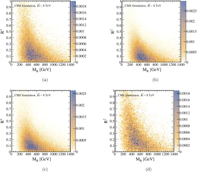
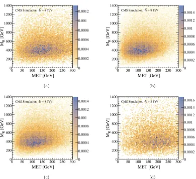
In the following section we will examine the effect of the branching ratios listed in Table 4.1

on the kinematics of the m˜_b = 600 GeV, m_χ_˜0

1 = 300 GeV model. If we examine Fig. 4.3, we see

that we obtain the MR shape in the desired range as predicted by M∆, as well asR2 peak values

in the desired range. As the branching ratio to ˜χ0

2 decreases, we see that the peak region is less

defined. Fig. 4.3d shows that theR2_versus_M

Rdistribution with the loosest clustering in the events

corresponds to the smallest branching ratio. This can be understood through the chance that the

event we capture is asymmetric.

With an 100% branching ratio to ˜χ02, we see a marked decrease in events at highR2. Because of

howR2 is defined withE/T dependence, largerE/T in general should result in a largerE/T if theMR

is fixed. The 2D distribution shrinks to lowerR2_{, although the}_M

R distribution, as expected, shifts

very little. However, regardless of the branching ratio, the plots still maintain a significant portion

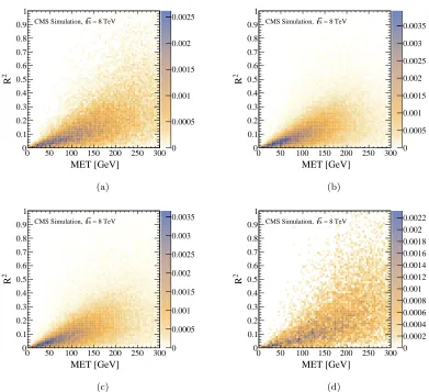
of events above R2 _≈₀_._{1. With Fig. 4.4, we see a similar phenomenon as the branching ratio to} ˜

χ0

2 increases. The plot shows the strong dependence of R2 on the E/T distribution. Although the

distribution becomes more defined, the rough slope of the R2 _vs_E_/

T 2D distribution remains the

same.

The MR versus E/T 2D plots reveal the robustness of the MR variable with varying branching

ratios. Comparing Fig. 4.4a and b shows that increasing the branching ratio clusters the events

(25)

0 0.0002 0.0004 0.0006 0.0008 0.001 0.0012 0.0014 0.0016 0.0018 [GeV] R M

0 200 400 600 800 1000 1200 1400

2 R 0 0.1 0.2 0.3 0.4 0.5 0.6 0.7 0.8 0.9 1

= 8 TeV s CMS Simulation, (a) 0 0.0005 0.001 0.0015 0.002 0.0025 [GeV] R M

0 200 400 600 800 1000 1200 1400

2 R 0 0.1 0.2 0.3 0.4 0.5 0.6 0.7 0.8 0.9 1

= 8 TeV s CMS Simulation, (b) 0 0.0005 0.001 0.0015 0.002 0.0025 [GeV] R M

0 200 400 600 800 1000 1200 1400

2 R 0 0.1 0.2 0.3 0.4 0.5 0.6 0.7 0.8 0.9 1

= 8 TeV s CMS Simulation, (c) 0 0.0002 0.0004 0.0006 0.0008 0.001 0.0012 0.0014 0.0016 0.0018 [GeV] R M

0 200 400 600 800 1000 1200 1400

2 R 0 0.1 0.2 0.3 0.4 0.5 0.6 0.7 0.8 0.9 1

= 8 TeV s CMS Simulation,

(d)

Figure 4.3: Z-axis scale units are such that the total number of events is normalized to 1. m˜_b= 600 GeV,mχ˜0

2 _versus_M

R for the 50% (to ˜χ02) working model. (b) R

2 _versus

MR for the 100% (to ˜χ02) working model. (c)R2versusMR for the 90% (to ˜χ02) working model. (d) R2 versusMRfor the 10% (to ˜χ02) working model.

also lose the nicely clustered peak since the decay of the ˜bpair is now mostly asymmetric. However,

theMR spread seems to change minimally.

The conclusion from this study of the branching ratios with this one mass working point is that

an increase in branching ratio to ˜χ0₂ is beneficial for anR2distribution that evades the current LHC

bounds. Varying the branching ratio has little effect on the MR. Furthermore, standard bottom

squark searches assume that the bottom squark decays directly to ˜χ01[33], so increasing the branching

ratio to ˜χ0

(26)

0 0.0005 0.001 0.0015 0.002 0.0025 MET [GeV]

0 50 100 150 200 250 300

2 R 0 0.1 0.2 0.3 0.4 0.5 0.6 0.7 0.8 0.9 1

= 8 TeV s CMS Simulation, (a) 0 0.0005 0.001 0.0015 0.002 0.0025 0.003 0.0035 MET [GeV]

0 50 100 150 200 250 300

2 R 0 0.1 0.2 0.3 0.4 0.5 0.6 0.7 0.8 0.9 1

= 8 TeV s CMS Simulation, (b) 0 0.0005 0.001 0.0015 0.002 0.0025 0.003 0.0035 MET [GeV]

0 50 100 150 200 250 300

2 R 0 0.1 0.2 0.3 0.4 0.5 0.6 0.7 0.8 0.9 1

= 8 TeV s CMS Simulation, (c) 0 0.0002 0.0004 0.0006 0.0008 0.001 0.0012 0.0014 0.0016 0.0018 0.002 0.0022 MET [GeV]

0 50 100 150 200 250 300

2 R 0 0.1 0.2 0.3 0.4 0.5 0.6 0.7 0.8 0.9 1

(d)

2 _versus_E_/

T , for the 50% (to ˜χ02) working model. (b)R2versus /

ET , for the 100% (to ˜χ02) working model. (c)R2 versusE/T , for the 90% (to ˜χ02) working model. (d)R2 _versus_E_/

(27)

0 0.0002 0.0004 0.0006 0.0008 0.001 0.0012 MET [GeV]

0 50 100 150 200 250 300

[GeV] R M 0 200 400 600 800 1000 1200 1400

0 50 100 150 200 250 300

[GeV] R M 0 200 400 600 800 1000 1200 1400

= 8 TeV s CMS Simulation, (b) 0 0.0002 0.0004 0.0006 0.0008 0.001 0.0012 0.0014 MET [GeV]

0 50 100 150 200 250 300

[GeV] R M 0 200 400 600 800 1000 1200 1400

= 8 TeV s CMS Simulation, (c) 0 0.0002 0.0004 0.0006 0.0008 0.001 0.0012 0.0014 0.0016 MET [GeV]

0 50 100 150 200 250 300

[GeV] R M 0 200 400 600 800 1000 1200 1400

(d)

1 = 300 GeV model. (a)MR versusE/T for the 50% (to ˜χ

0

2) working model. (b)MRversus

/

(28)

4.7 Mass Splitting Study with Fixed

χ

˜

0₁

Mass

The next parameter that would affect the kinematics is the mass splitting of the system, i.e. the

difference in mass between the bottom squark and lightest neutralino. We can classify this in two

ways: usingM∆, or simplyMsplit=m˜b−mχ˜0

1. The following subsections investigate the kinematics

of models with the characteristics listed in Table 4.2. Notice the caveat that these effects would not

necessarily be decoupled from the effects of changing the bottom squark mass.

m

˜_b

m

χ˜0

2

m

χ˜

0

1

M

∆

M

split

BR (to ˜

χ

0 2

)

550 GeV

430 GeV

300 GeV

386.36 GeV

250 GeV

90%

450 GeV

430 GeV

300 GeV

250 GeV

150 GeV

100%

530 GeV

430 GeV

300 GeV

360.19 GeV

230 GeV

100%

Table 4.2: Table of the models investigated in the mass splitting study, with their associated values ofM∆andMsplit.

The 1DE/T distributions have a strong dependence on mass splitting since with a smaller mass

splitting there is likely less energy available for the decay particles (Fig. 4.10a. With Figures 4.6,

4.7, 4.8, we can also see a strong dependence of MR on M∆. This is in line with the principle

that MR is an estimator of M∆. If we compare Figure 4.6b to Figure 4.4c, theR2 versus E/T 2D

distributions are roughly the same, indicating that the decrease in mass splitting from them˜_b= 600

GeV model to the m˜_b = 550 GeV has a relatively small effect on these variables. However, when

we look at Figure 4.7b, we notice a large difference not only in a tighter clustering at smallE/T,R2,

but also a change in the slope for them˜_b = 450 GeV model. From Figure 4.7c, we also notice that

theMRclusters at a center of less than 200 GeV, which is lower than we would expect. There is an

unexpected shift of the peaks of the MR distributions if we compare the various models in Figure

(29)

0 0.0005 0.001 0.0015 0.002 0.0025 0.003 [GeV] R M

0 200 400 600 800 1000 1200 1400

2 R 0 0.1 0.2 0.3 0.4 0.5 0.6 0.7 0.8 0.9 1

= 8 TeV s CMS Simulation, (a) 0 0.0005 0.001 0.0015 0.002 0.0025 0.003 0.0035 0.004 MET [GeV]

0 50 100 150 200 250 300

2 R 0 0.1 0.2 0.3 0.4 0.5 0.6 0.7 0.8 0.9 1

= 8 TeV s CMS Simulation, (b) 0 0.0002 0.0004 0.0006 0.0008 0.001 0.0012 0.0014 0.0016 0.0018 MET [GeV]

0 50 100 150 200 250 300

[GeV] R M 0 200 400 600 800 1000 1200 1400

(c)

Number of Jets

0 1 2 3 4 5 6 7 8 9

a.u 0 0.05 0.1 0.15 0.2 0.25 0.3

(d)

Figure 4.6: Characterization of them˜_b= 550 GeV,m_χ_˜0

0

2. Z-scale units are such that the total number of events is normalized to 1. (a)R2_versus_M

R. (b)R2 versus

/

ET . (c)MR versusE/T . (d) Number of PF jets, clustered with the anti-kT algorithm with ∆R =

(30)

0 0.0005 0.001 0.0015 0.002 0.0025 0.003 0.0035 0.004 0.0045 [GeV] R M

0 200 400 600 800 1000 1200 1400

2 R 0 0.1 0.2 0.3 0.4 0.5 0.6 0.7 0.8 0.9 1

0 50 100 150 200 250 300

2 R 0 0.1 0.2 0.3 0.4 0.5 0.6 0.7 0.8 0.9 1

= 8 TeV s CMS Simulation, (b) 0 0.0005 0.001 0.0015 0.002 0.0025 0.003 0.0035 0.004 MET [GeV]

0 50 100 150 200 250 300

[GeV] R M 0 200 400 600 800 1000 1200 1400

(c)

Number of Jets

0 1 2 3 4 5 6 7 8 9

a.u 0 0.05 0.1 0.15 0.2 0.25 0.3 0.35

(d)

0

R. (b)R2 versus

/

(31)

0 0.0005 0.001 0.0015 0.002 0.0025 0.003 0.0035 [GeV] R M

0 200 400 600 800 1000 1200 1400

2 R 0 0.1 0.2 0.3 0.4 0.5 0.6 0.7 0.8 0.9 1

= 8 TeV s CMS Simulation, (a) 0 0.001 0.002 0.003 0.004 0.005 MET [GeV]

0 50 100 150 200 250 300

2 R 0 0.1 0.2 0.3 0.4 0.5 0.6 0.7 0.8 0.9 1

= 8 TeV s CMS Simulation, (b) 0 0.0002 0.0004 0.0006 0.0008 0.001 0.0012 0.0014 0.0016 0.0018 0.002 0.0022 MET [GeV]

0 50 100 150 200 250 300

[GeV] R M 0 200 400 600 800 1000 1200 1400

(c)

Number of Jets

0 1 2 3 4 5 6 7 8 9

a.u 0 0.05 0.1 0.15 0.2 0.25

0.3 CMS Simulation, s = 8 TeV

(d)

Figure 4.8: Characterization of them˜_b= 530 GeV,mχ˜0

0

R. (b)R2 versus

/

0.5.

In an effort to decipher these effects, we can think of howMRis defined. SinceMRis constructed

from jets and particles that must have a minimum pT, soft particles will be excluded. In Figure

4.11, we see that the available energy to impart to the bottom quark is only 20 GeV; thus, these

b-jets are likely very soft. As a result, they are not clustered in the hemispheres that go into the

calculation ofMR, andM∆is not being constructed accurately. SinceR=MTR/MR, this also affects

the distribution of R2. A smallerMR than expected thus increases the slope of theR2 versus E/T

plot.

This explanation is further supported by the plot of the distribution of PF jets that enter the

hemispheres (see Figure 4.7d), which has a mode of only two jets. We expect on average four jets

for a model with BR = 100% to ˜χ0

2, with two from the direct decay of the bottom squark particle

(32)

[GeV]

R

M

0 200 400 600 800 10001200140016001800

a.u 0 0.01 0.02 0.03 0.04 0.05 0.06 0.07

0.08 _{= 300}

χ∼ = 450 m

b ~

m

= 300 χ∼ = 550 m

b ~

m

= 300 χ∼ = 530 m

b ~

m = 8 TeV s CMS Simulation,

(a)

2

R

0 0.2 0.4 0.6 0.8 1 1.2 1.4

a.u -4 10 -3 10 -2 10 -1 10 = 300 χ∼ = 450 m

b ~

m

= 300 χ∼ = 550 m

b ~

m

= 300 χ∼ = 530 m

b ~

(b)

Figure 4.9: Razor variable distributions for the various mass splitting with fixed ˜χ01 mass. (a)MR

1D distributions. (b)R2 _{1D distributions.}

MET [GeV]

0 100 200 300 400 500 600 700 800

a.u 0 0.02 0.04 0.06 0.08 0.1 = 300 χ∼ = 450 m

b ~

m

= 300 χ∼ = 550 m

b ~

m

= 300 χ∼ = 530 m

b ~

(a)

[GeV]

T

Leading Jet p

0 100 200 300 400 500 600 700 800 900 1000

a.u 0 0.02 0.04 0.06 0.08

0.1 mb~ = 450 mχ∼ = 300

= 300 χ∼ = 550 m

b ~

m

= 300 χ∼ = 530 m

b ~

(b)

Figure 4.10: Kinematic distributions for the various mass splitting with fixed ˜χ0

1 mass. (a)E/T 1D

distributions. (b) Leading jetpT 1D distributions (excluding H→ b¯bjets).

them˜_b= 450 GeV model is shown to be very soft in Figure 4.10b.

Following the m˜_b = 450 GeV model, the m˜_b = 530 GeV model was investigated. Here, we see

that although the mass splitting is smaller, the slope of the R2 _versus _E_/

T plot does not increase

dramatically (Figure 4.8b). Thus, we can conclude that there is a threshold of mass splitting in

between 530 GeV and 450 GeV, mostly likely around≈460 GeV, in which the b-jets are too soft to be included in the calculation of MR. The number of jets in Figure 4.8d is also as expected, and

MR returns to being a good probe forM∆(Figure 4.8c).

In conclusion, decreasing the mass splitting changes the MR as expected, but has little effect on

theR2 _{up to a certain threshold. After the b-jets are too soft to be included in the calculation of}

(33)

Figure 4.11: The decay spectrum for them˜_b= 450 GeV model.

4.8 Mass Splitting Study with Fixed

˜

b

Mass

m

˜_b

m

χ˜0

2

m

χ˜

0

1

M

∆

M

split

BR (to ˜

χ

0 2

)

600 GeV

230 GeV

100 GeV

583.33 GeV

500 GeV

100%

600 GeV

330 GeV

200 GeV

533.33 GeV

400 GeV

100%

600 GeV

430 GeV

300 GeV

450 GeV

300 GeV

100%

Table 4.3: Table of the models investigated in the mass splitting study with fixed ˜b mass, and their associated values ofM∆ andMsplit.

Varying the mass splitting by changing the ˜χ01mass has a different effect than varying the ˜bmass.

We see that larger mass splitting corresponds to largerMRvalues, as expected, but causesR2to fall

faster (Fig. 4.14). The 2DR2_versus_M

Rdistribution is also clustered more tightly around the peak

values (Fig. 4.13a, 4.12a). This is due to an increasing MR accompanied by a relatively constant

/

ET distribution in Figure 4.15a. Although the larger mass splitting correlates with a larger leading

jetpT (Fig. 4.15b), which we expect is the b quark directly decaying from the bottom squark, the

˜ χ0

1 pT decreases with larger mass splitting. Furthermore, we can see a dependence of the azimuthal

angle, ∆Φ, between the two ˜χ0

1 particles. The 2DMR versusE/T distribution becomes more spread

out with larger mass splitting (Fig. 4.13c, 4.12c).

We note that the original squarks are almost always produced back-to-back in ∆Φ, regardless

of the mass splitting (Fig. 4.17b). Also note that as the leading jetpT increases, the ˜χ01 particles

will most likely deviate more from the path of the original bottom squark due to the recoil of the

˜ χ0

1 from the Higgs, which are produced from ˜χ02 particles recoiling against the b quarks. The larger

the mass splitting, the larger the leading jet pT, and the more the ˜χ01 particles deviate from the

original path of the bottom squark. This is illustrated in the ˜χ0

1 ∆Φ distributions in Figure 4.16b.

The smaller mass splitting correlates with the ˜χ0

1particles being produced more often back-to-back

(34)

0 0.0005 0.001 0.0015 0.002 0.0025 [GeV] R M

0 200 400 600 800 1000 1200 1400

2 R 0 0.1 0.2 0.3 0.4 0.5 0.6 0.7 0.8 0.9 1

0 50 100 150 200 250 300

2 R 0 0.1 0.2 0.3 0.4 0.5 0.6 0.7 0.8 0.9 1

= 8 TeV s CMS Simulation, (b) 0 0.0002 0.0004 0.0006 0.0008 0.001 0.0012 MET [GeV]

0 50 100 150 200 250 300

[GeV] R M 0 200 400 600 800 1000 1200 1400

(c)

Number of Jets

0 1 2 3 4 5 6 7 8 9

a.u 0 0.05 0.1 0.15 0.2 0.25

(d)

1= 200 GeV model with 100% to ˜χ

0

R. (b)R2 versus

/

0.5.

Even though a smaller mass splitting has less energy available to the ˜χ0

1, its effect is overshadowed

by the explanation that the ˜χ0

1particles likely have morepT if they remain on the path of the original

bottom squark. Examining Figure 4.16a, we see that a smaller mass splitting results in higher leading

˜

χ0₁pT. However, this higher leading ˜χ01pT is balanced by the effect that the ˜χ01particles are produced

more often back-to-back in ∆Φ with a smaller mass splitting. As a result, theE/T distribution stays

roughly constant due to the two ˜χ01momentum vectors canceling each other. Overall, this effect can

be attributed to the two-step decay chain.

This phenomena was not present in Section 4.7. In the previous section, any effects from variable

sampling the √s distribution due to the production of bottom squarks of different masses were not removed. This likely counteracted the effect of the particle decay angles, resulting in a E/T

(35)

0 0.0005 0.001 0.0015 0.002 0.0025 0.003 0.0035 [GeV] R M

0 200 400 600 800 1000 1200 1400

2 R 0 0.1 0.2 0.3 0.4 0.5 0.6 0.7 0.8 0.9 1

= 8 TeV s CMS Simulation, (a) 0 0.001 0.002 0.003 0.004 0.005 0.006 MET [GeV]

0 50 100 150 200 250 300

2 R 0 0.1 0.2 0.3 0.4 0.5 0.6 0.7 0.8 0.9 1

= 8 TeV s CMS Simulation, (b) 0 0.0002 0.0004 0.0006 0.0008 0.001 0.0012 MET [GeV]

0 50 100 150 200 250 300

[GeV] R M 0 200 400 600 800 1000 1200 1400

(c)

Number of Jets

0 1 2 3 4 5 6 7 8 9

a.u 0 0.05 0.1 0.15 0.2 0.25

(d)

0

R. (b)R2 versus

/

0.5.

soft due to the relatively smaller mass splittings, which also minimizes the effect of the particle decay

angles.

In summary: for the larger mass splitting models, the R2 _{distribution is desirable but the} _M

R

(36)

[GeV]

R

M

0 200 400 600 800 10001200140016001800

a.u 0 0.01 0.02 0.03 0.04 0.05 = 300 χ∼ = 600 m

b ~

m

= 200 χ∼ = 600 m

b ~

m

= 100 χ∼ = 600 m

b ~

(a)

2

R

0 0.2 0.4 0.6 0.8 1 1.2 1.4

a.u -5 10 -4 10 -3 10 -2 10 -1 10 = 300 χ∼ = 600 m

b ~

m

= 200 χ∼ = 600 m

b ~

m

= 100 χ∼ = 600 m

b ~

(b)

Figure 4.14: Razor variable distributions for the various mass splitting with fixed ˜b mass. (a) MR

1D distributions. (b)R2 1D distributions.

MET [GeV]

0 100 200 300 400 500 600 700 800

a.u 0 0.01 0.02 0.03 0.04 0.05 0.06 = 300 χ∼ = 600 m

b ~

m

= 200 χ∼ = 600 m

b ~

m

= 100 χ∼ = 600 m

b ~

(a)

[GeV]

T

Leading Jet p

0 100 200 300 400 500 600 700 800 900 1000

a.u 0 0.01 0.02 0.03 0.04 0.05 0.06 0.07

0.08 mb~ = 600 mχ∼ = 300

= 200 χ∼ = 600 m

b ~

m

= 100 χ∼ = 600 m

b ~

(b)

Figure 4.15: Kinematic distributions for the various mass splitting with fixed ˜b mass. (a) E/T 1D

(37)

[GeV]

T

Leading LSP p

0 100 200 300 400 500 600 700 800 900 1000

a.u 0 0.01 0.02 0.03 0.04 0.05 0.06 0.07 0.08 = 300 χ∼ = 600 m

b ~

m

= 200 χ∼ = 600 m

b ~

m

= 100 χ∼ = 600 m

b ~

m = 8 TeV s CMS Simulation, (a) Φ ∆ LSP

-3 -2 -1 0 1 2 3

a.u 0 0.01 0.02 0.03 0.04 0.05

0.06 _{= 300}

χ∼ = 600 m

b ~

m

= 200 χ∼ = 600 m

b ~

m

= 100 χ∼ = 600 m

b ~

(b)

Figure 4.16: ˜χ01kinematic distributions for the various mass splitting with fixed ˜bmass. (a) Leading ˜

χ01 pT 1D distributions. (b) ∆Φ between the two ˜χ01 particles.

[GeV] T p b ~ Leading

0 100 200 300 400 500 600 700 800 900 1000

a.u 0 0.005 0.01 0.015 0.02 0.025 0.03 = 300 χ∼ = 600 m

b ~

m

= 200 χ∼ = 600 m

b ~

m

= 100 χ∼ = 600 m

b ~

m = 8 TeV s CMS Simulation, (a) Φ ∆ b ~

-3 -2 -1 0 1 2 3

a.u 0 0.02 0.04 0.06 0.08 0.1 0.12 0.14 0.16 0.18

0.2 _{= 300}

χ∼ = 600 m

b ~

m

= 200 χ∼ = 600 m

b ~

m

= 100 χ∼ = 600 m

b ~

(b)

(38)

4.9 ˜

b

Mass Study with Fixed

M

∆

In the following models, we instead vary the bottom squark mass while keeping M∆ roughly the

same. The model characteristics are given in Table 4.4.

Name

m

˜_b

m

χ˜0

2

m

χ˜01

M

∆

M

split

BR (to ˜

χ

0 2

)

CLT2015-AW1

470 GeV

230 GeV

100 GeV

448.72 GeV

370 GeV

100%

CLT2015-AW2

500 GeV

290 GeV

160 GeV

448.8 GeV

340 GeV

100%

CLT2015-AW3

600 GeV

430 GeV

300 GeV

450 GeV

300 GeV

100%

Table 4.4: Table of the models investigated in the bottom squark mass study, with their associated values ofM∆ andMsplit.

We see an deficit of events in the R2 _{tail in the smaller ˜}_b _{mass samples (Figures 4.18a, 4.19a,}

4.21), as compared to the m˜_b = 600 GeV model. TheR2 _versus _M

R distribution for the ˜b = 470

model exhibits very low, clusteredR2_{events, as well as a tightly clustered}_R2_versus_E_/

T distribution

(see Figure 4.18b). As a result, this model is promising for our desired constraints. From this point,

we will refer to it as theCLT2015-AW1model for convenience. The other two models,m˜_b= 500

GeV andm˜_b= 600 GeV, will be calledCLT2015-AW2andCLT2015-AW3, respectively.

This small R2 tail is likely a mixture of the phenomena from the previous two studies, since we

have neither fixed ˜bnor fixed ˜χ01 masses. However, the deficit ofR2events seems to be more similar

to the fixed ˜bmass study. More energy is available for the b quark (Figure 4.20), which is exhibited

in the higher leading jetpT if we compare Figures 4.23a and 4.10b, which increases the role of the

angles of decay in the kinematics. We again have a ˜χ0

1 ∆Φ distribution that varies greatly between

the different models (Figure 4.23d). The model with the smallest mass splitting, CLT2015-AW3,

again has the most back-to-back ˜χ0

(39)

0 0.0005 0.001 0.0015 0.002 0.0025 0.003 0.0035 0.004 0.0045 [GeV] R M

0 200 400 600 800 1000 1200 1400

2 R 0 0.1 0.2 0.3 0.4 0.5 0.6 0.7 0.8 0.9 1

0 50 100 150 200 250 300

2 R 0 0.1 0.2 0.3 0.4 0.5 0.6 0.7 0.8 0.9 1

= 8 TeV s CMS Simulation, (b) 0 0.0002 0.0004 0.0006 0.0008 0.001 0.0012 0.0014 0.0016 0.0018 MET [GeV]

0 50 100 150 200 250 300

[GeV] R M 0 200 400 600 800 1000 1200 1400

(c)

Number of Jets

0 1 2 3 4 5 6 7 8 9

a.u 0 0.05 0.1 0.15 0.2 0.25

(d)

0

R. (b)R2 versus

/

(40)

0 0.0005 0.001 0.0015 0.002 0.0025 0.003 0.0035 [GeV] R M

0 200 400 600 800 1000 1200 1400

2 R 0 0.1 0.2 0.3 0.4 0.5 0.6 0.7 0.8 0.9 1

= 8 TeV s CMS Simulation, (a) 0 0.001 0.002 0.003 0.004 0.005 0.006 MET [GeV]

0 50 100 150 200 250 300

2 R 0 0.1 0.2 0.3 0.4 0.5 0.6 0.7 0.8 0.9 1

= 8 TeV s CMS Simulation, (b) 0 0.0002 0.0004 0.0006 0.0008 0.001 0.0012 0.0014 0.0016 MET [GeV]

0 50 100 150 200 250 300

[GeV] R M 0 200 400 600 800 1000 1200 1400

(c)

Number of Jets

0 1 2 3 4 5 6 7 8 9

a.u 0 0.05 0.1 0.15 0.2 0.25

(d)

0

R. (b)R2 versus

/

0.5.

(41)

[GeV]

R

M

0 200 400 600 800 10001200140016001800

a.u 0 0.01 0.02 0.03 0.04 0.05

= 470 GeV

b ~

m

= 500 GeV

b ~

m

= 600 GeV

b ~

m

(a)

2

R

0 0.2 0.4 0.6 0.8 1 1.2 1.4

a.u -5 10 -4 10 -3 10 -2 10 -1 10

= 470 GeV

b ~

m

= 500 GeV

b ~

m

= 600 GeV

b ~

m

(b)

Figure 4.21: Razor variable distributions for the various ˜b models with fixed M∆. (a) MR 1D

distributions. (b)R21D distributions.

[GeV]

T

Leading Jet p

0 100 200 300 400 500 600 700 800 900 1000

a.u 0 0.01 0.02 0.03 0.04 0.05 0.06 0.07

0.08 mb~ = 470 GeV

= 500 GeV

b ~

m

= 600 GeV

b ~

m

(a)

[GeV]

T

Subleading Jet p

0 100 200 300 400 500 600 700 800 900 1000

a.u 0 0.02 0.04 0.06 0.08 0.1 0.12

= 470 GeV

b ~

m

= 500 GeV

b ~

m

= 600 GeV

b ~

m

(b)

[GeV]

T

Leading LSP p

0 100 200 300 400 500 600 700 800 900 1000

a.u 0 0.02 0.04 0.06 0.08

0.1 mb~ = 470 GeV

= 500 GeV

b ~

m

= 600 GeV

b ~

m

(c)

[GeV]

T

Subleading LSP p

0 100 200 300 400 500 600 700 800 900 1000

a.u 0 0.02 0.04 0.06 0.08 0.1

= 470 GeV

b ~

m

= 500 GeV

b ~

m

= 600 GeV

b ~

m

(d)

Figure 4.22: Kinematic distributions for the various ˜bmodels with fixedM∆. (a) Leading jetpT 1D

distributions (excluding H→ b¯b jets). (b) Subeading jetpT 1D distributions (excluding H → b¯b

(42)

[GeV] T p b ~ Leading

0 100 200 300 400 500 600 700 800 900 1000

a.u 0 0.005 0.01 0.015 0.02 0.025 0.03 0.035 0.04

= 470 GeV

b ~

m

= 500 GeV

b ~

m

= 600 GeV

b ~

m

= 8 TeV s CMS Simulation, (a) [GeV] T p b ~ Subleading

0 100 200 300 400 500 600 700 800 900 1000

a.u 0 0.01 0.02 0.03 0.04

0.05 mb~ = 470 GeV

= 500 GeV

b ~

m

= 600 GeV

b ~

m

= 8 TeV s CMS Simulation, (b) Φ ∆ b ~

-3 -2 -1 0 1 2 3

a.u 0 0.02 0.04 0.06 0.08 0.1 0.12 0.14 0.16 0.18

0.2 _{= 470 GeV}

b ~

m

= 500 GeV

b ~

m

= 600 GeV

b ~

m

= 8 TeV s CMS Simulation, (c) Φ ∆ LSP

-3 -2 -1 0 1 2 3

a.u 0 0.01 0.02 0.03 0.04 0.05

0.06 _{= 470 GeV}

b ~

m

= 500 GeV

b ~

m

= 600 GeV

b ~

m

(d)

Figure 4.23: Kinematic distributions for the various ˜b models with fixed M∆. (a) Leading ˜b pT

1D distributions. (b) Subleading ˜b pT 1D distributions. (c) ∆Φ between the two bottom squarks

New Physics Models in the Diphoton Final State at CMS