IJPAS Vol.03 Issue-12, (December, 2016) ISSN: 2394-5710 International Journal in Physical & Applied Sciences (Impact Factor- 4.657)

(1)

A Monthly Double-Blind Peer Reviewed Refereed Open Access International e-Journal - Included in the International Serial Directories International Journal in Physical & Applied Sciences

http://www.ijmr.net.in email id- [email protected]

Heat and Mass Transfer of Unsteady MHD Flow of a Perfect Conducting Bi-viscosity Fluid through a Porous Medium

by

Abeer A. Shaaban(1, 2) and Khaled Elagamy(1, 3)

1) Department of Mathematics, Faculty of Education, Ain Shams University, Roxy, Cairo, Egypt

2) Department of Management Information Systems, Faculty of Business Administration in Rass, Al Qassim University, Al Qassim, KSA

3) Department of Mathematics, Faculty of Science in Al-Bukayriyah, Al Qassim University, Al Qassim, KSA

Abstract

In this paper, we examine the unsteady boundary layer MHD flow of a perfect conducting incompressible non-Newtonian fluid of type Bi-viscosity with heat and mass transfer over a vertical infinite plate through a porous medium in the presence of an induced magnetic field. The influences of non-Newtonian dissipation and thermal diffusion are taken in our consideration. The governing partial differential equations with the appropriate boundary conditions are reduced to ordinary differential equations by using the Lightill’s perturbation technique. The solutions of the resulting non-linear ODEs are obtained numerically by using the Explicit Finite-Difference method and showed graphically under the effects of the physical parameters of the problem through a set of figures.

(2)

International Journal in Physical & Applied Sciences (Impact Factor- 4.657)

http://www.ijmr.net.in email id- [email protected] 1- Introduction:

In recent years, the effects of magnetic field have important applications in physics, chemistry and engineering. there is an increasing interest in magnetohydrodynamics (MHD) flows for fluid through porous media, because of its numerous applications in geophysics and energy related problems, such as thermal insulation of balding.

(Bestman and Adjepong, 1998) studied the unsteady hydromagnetic free convection flow with radiative heat transfer in a rotating fluid. The study of MHD free convection and mass transfer flow through a porous medium was considered by (Jha, 1991), whose didn’t consider the effect of radiation. (Ram and Jain, 1990) presented a study of hydromagnetic Ekam layer on convective heat generating fluid in slip flow regime.

Also, (Chamkha, 2004) investigated the unsteady convective heat and mass transfer past a semi-infinite permeable moving plate with heat absorption. In another recent study, (Ibrahim et al., 2004) investigated the unsteady magnetohydrodynamic micro-polar fluid flow and heat transfer over a vertical porous plate through a porous medium in the presence of thermal and mass diffusion with a constant heat source. (Chamkha, 2004) and (Cookey et al., 2003) give a good review on MHD flows through a porous medium, ( Ezzat et al., 2011) studied the problem of combined heat and mass transfer of a perfect conducting micropolar fluid in MHD natural convection adjacent to an infinite vertical surface. (Hayat et al., 2004) found the exact solutions of flow problems of an Oldroyd-B fluid.

The objective of this work is to investigate the numerical solution by using the Explicit Finite Difference method (Saxena, 1991) for the system of non-linear ordinary differential equations which arises from the problem of MHD mixed convection flow of a perfect conducting non-Newtonian fluid with thermal relaxation time. We obtained the Numerical results of the velocity, the temperature, the concentration, and the magnetic field in terms of the dimensionless distance

y

for different values of various non-dimensional parameters. The results are shown graphically and discussed in detail.

2- Formulation of the problem

(3)

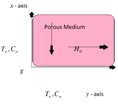
http://www.ijmr.net.in email id- [email protected] Fig. (1): Sketch of the problem

x- axis

Porous Medium

Tw,Cw H0

g

T



,

C



y

- axis

Suppose that a constant magnetic field of strength H0 acts in the direction parallel to the

y

-

axis, this produced an induced magnetic field

h



(

h

,

0 ,

0 )

and induced electric field

E



(

0 ,

E

)

as

well as a conduction current density

J



(

0 ,

J

)

which satisfy the linearized equations of electromagnetism valid for slowly media for a perfect conductor. The chosen model of the non-Newtonian fluid is the Bi-viscosity model, which is in the usual notation:





















,

)

2 (

2 ,

)

2 (

2

c ij c y c ij y ij

e

P

e

P











  (1)

where



_ is the plastic viscosity, Py is the yielding stress and



eijeij,

(

)

2

1

i j j i ij

x

u

x

u

e









y

P









_

2

, (2)

Under the above assumptions, the governing equations of the problem may be written as:

), ( ) 1 ( ) ( ) ( 0 0 0 2 2 1 t E y h H u k y u C C g T T g t u C T _                   

_













(3)

, ) ( ) 1 ( ) 1 ( 2 1 2 2 0 y u c y T c t T

t _p _p 

           













(4)

,

)

1 (

₂ 2 2 2 0

y

T

D

K

y

C

D

t

C

t

c

m m T m p

_















(4)

http://www.ijmr.net.in email id- [email protected] ), ( ₀ t E J y h       

_

(6) , 0 t h y E      

_

(7) , 0 0H u

E 



(8)

, 0    y h (9)

Where u is the fluid velocity in the x- direction,

t

is the time,

g

is the acceleration due to gravity,



0 is the relaxation time,



0 is the electric permeability,



0 is the magnetic permeability,

T



is the thermal expansion coefficient,



C is the concentration expansion coefficient,



is the electric conductivity,



is the fluid density, k is the permeability coefficient,



_ is the plastic

viscosity,

y

P









_

2

is the upper limit of viscosity coefficient,

T

is the temperature,



is the

thermal conductivity,

c

p is the specific heat at constant pressure, C denotes the concentration, Dm

is the coefficient of mass diffusivity,

K

_T is the thermal diffusion ratio and Tm is the mean fluid temperature.

The appropriate boundary conditions are

0

, ,

,

0 T T C C h H

u  w  w  at

y



0

(10)

0 ,

,

0 



T

_

C

_

h

u

as y (11)

To reduce the above equations into non-dimensional form, let us introduce the following dimensionless variables                  C C C C C T T T T T J H J H E E H h h t t y y u u w w * * 0 * 0 0 * 0 * 0 2 * 0 2 * * * , , , , , , , ,

























(12)

The equations (3) - (9) with the boundary conditions (10) and (11) after introducing the non – dimensional variables and dropping the star mark (*) become

, 1 ) 1 ( ) 1 ( ₂ 2 1 2 2 y h u K y u C G T G t u

c T C 

           



_

 (13)

,

)

(

)

1 (

1 )

1 (

₂ 1 2

2 0

y

u

E

y

T

P

t

T

t

_r c



(5)

,

1 )

1 (

2 2 2 2 0

y

T

S

y

C

S

t

C

t

_c r















(15)

,

2 2

t

u

c

J

y

h













(16)

With the boundary conditions

1 ,

0 



T

C

h

u

at

y



0

(17)

0 ,

0 



T

C

h

u

as y (18)

Where ( ₃ )

U T T g

G T l u

T









 is the thermal Grashof number, ( ₃ )

U C C g

G C l u

c









 is mass

Grashof number, ₂

2



k U

K  is the permeability parameter,





p r

c

P  is the Prandtl number,

) ( 2 u l p c T T c U E 

 is the Eckert number,

m c

D

S 



is the Schimdt number and

) ( ) ( u l m u l T m r C C T T T K D S   

is the Soret number,

3- Method of solution

In order to solve the system of partial differential equations (13) – (16), subjected to the boundary conditions (17) and (18), we consider the following Lightill’s perturbation technique

, ) ( ) ( ) , ( , ) ( ) ( ) , ( , ) ( ) ( ) , ( , ) ( ) ( ) , ( 1 0 1 0 1 0 1 0 t i t i t i t i e y h y h t y h e y C y C t y C e y T y T t y T e y u y u t y u             (19)

Substituting (19) into the equations (13) – (16) with the boundary conditions (17) and (18), we get the following system of ordinary differential equations

),

(

'

)

(

)

(

)

(

1 )

(

''

)

1 (

0 0 0 0

1

y

h

y

C

G

y

T

G

y

u

K

y

u







T o



C





_

 (20) , 0 ) ( ' ) 1 ( ) ( '

' 0 2

1     y u E P y

To r c



(21)

, 0 ) ( ' ' ) ( '

' y S S T y 

C_o _c _r _o (23)

, ) ( '

0 y J

h  (24)

), ( ' ) ( ) ( ) ( ) 1 ( ) ( ' ' ) 1

( ₂ ₁ ₁ ₁ ₁

2 1 1 y h y C G y T G y u c i K i y

u     _T  _C 

(6)

http://www.ijmr.net.in email id- [email protected] , 0 ) ( ' ) ( ' ) 1 ( 2 ) ( ) ( ) (

'' ₀ 2 ₁ 1 ₀ ₁

1     

 y u y u E P y T P i y

T





_r _r _c



(26)

,

0 )

(

'

)

(

)

(

)

(

'

₀ 2 ₁ ₁

1

y





i

S

C

y



S

T

y



C





_c _c _r (27)

),

(

'

1 )

(

1

u

y

i

y

h





(28)

With the boundary conditions:

, 0 ) 0 ( , 0 ) 0 ( , 0 ) 0 ( , 1 ) 0 ( , 1 ) 0 ( , 1 ) 0 ( , 0 ) 0 ( ) 0

( ₁ ₀ ₀ ₀ ₁ ₁ ₁

0 u  T  C  h  T  C  h 

u (29)

, 0 1 1 1 0 0 0 1

0 u T C h T C h 

u as y (30)

The system of non-linear ordinary differential (20) – (28) together with the boundary conditions (29, 30), will be solved numerically by using the Explicit Finite-Difference method.

4- Numerical solution

The equations (20) – (28) can be written after applied explicit finite difference schemes (Saxena, 1991) as:



1



 

1 2 [ ] [ 1] 1

 

[] [ ] 0

 

0[ 1] 0

0 0 0 2 0 0 0 1 _                         h i h i h i C G i T G i u K h i u i u i u C T



,

 

_

_

 

0 ] 1 [ 1 ] 1 [ ] [ 2

1 1 ₀ ₀ 2

2 0 0

0 _ 

                    h i u i u E P h i T i T i T c

r



,

 

0 ] 1 [ ] [ 2 1 ] 1 [ ] [ 2 1 2 0 0 0 2 0 0

0 

                    h i T i T i T S S h i C i C i C r c ,

 

0 ]

1 [

0



















J

h

i

h

i

h

,



1



 

1

2 [

]

[

1 ]

(

1 )

 

[

]

[

]

1

 

1

[

1 ]

0

1 1 1 2 2 2 1 1 1 1













































h

i

h

i

h

i

C

G

i

T

G

i

u

c

i

K

i

h

i

u

i

u

i

u

C T







,

 

_

_

 

0 ]

1 [

]

1 [

1

2 ]

[

)

(

]

1 [

]

[

2

1

1 ₀ ₀ ₁ ₁

1 2 0 2 1 1

1

_























































h

i

u

i

u

h

i

u

i

u

E

P

i

T

P

i

h

i

T

i

T

i

T

c r r







,

 

0 ]

1 [

]

[

2

1 ]

[

)

(

]

1 [

]

[

2

1

2 1 1 1 1 2 0 2 1 1

1

















































h

i

T

i

T

i

T

S

i

C

S

i

h

i

C

i

C

i

C

r c c





,

 

1 1

 

1[ 1] 0

1 

        h i u i u i i h

(7)

where the index

i

refers to

y

and the



y



h



0 .

04

. According to the boundary conditions (29, 30) we can solved equations (31) numerically, then a Newtonian iteration method continues until either of goals specified by accuracy goal or precision goal is achieved.

5- Results and Discussion

In this paper we generalized the problem of the effects of thermal diffusion and non-Newtonian dissipation on the unsteady MHD flow of non- Newtonian fluid of type Bi-viscosity over a vertical plate in the presence of a varying magnetic field. The obtained non-linear ODEs describe the fluid velocity u, the fluid temperature

T

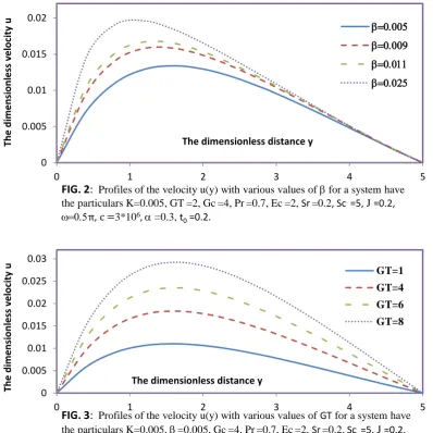
, the fluid concentration Cand the induced magnetic field h have been solved numerically by using the Explicit Finite-Difference method. The effects of the parameters controlled the problem are illustrated graphically as shown in figures (2 – 21) for different values.

Figure (2) shows the distribution of the velocity profile at different values of the upper limit of viscosity coefficient



. It is noted that, by increasing of



, the velocity increases. Figures (3 – 5)

describe the effect of the thermal Grashof number

G

_Ton the distributions of the velocity, the

temperature, and the concentration respectively. It is seen that, by increasing of

G

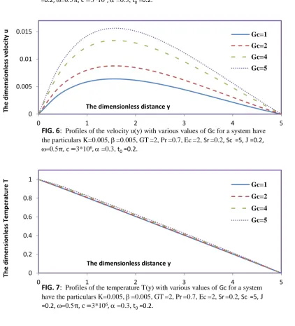
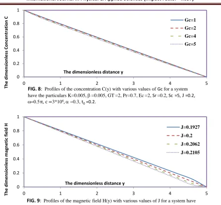
_T , the velocity and the temperature increase, but the concentration decreases. Figures (6 – 8) illustrate the effect of the mass Grashof number GC on the distributions of the velocity, the temperature, and the

concentration respectively. It is noted that, by increasing of GC, the velocity and the temperature increase, but the concentration decreases.

Figure (9) shows the effect of current density Jon the magnetic field. It is clear that, the magnetic field decreases by increasing of J.

Figures (10 – 12) illustrate the effect of the permeability parameter

K

on the velocity, The temperature, and the concentration respectively. It is seen that, by increasing of

K

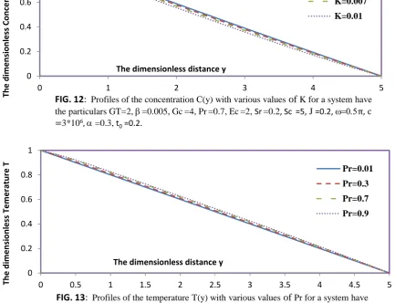
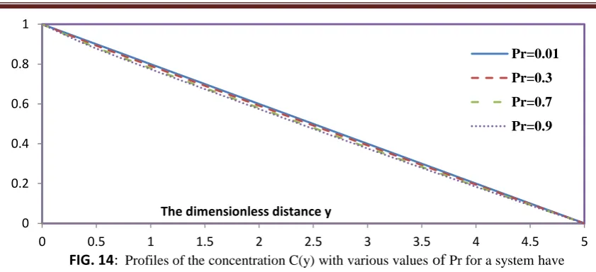
, the velocity and the temperature increase, but the concentration decreases.

Figures (13, 14) show the effect of Prandtl number

P

_r on the temperature, and concentration

profiles, respectively. It is seen that, the temperature increases by increasing of

P

_r, but the

concentration decreases by increasing of

P

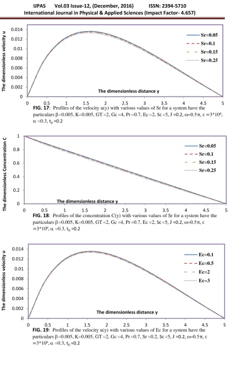
_r.

Figures (15, 16) illustrate the effect of Schimdt number Sc on the velocity and the concentration

respectively. It is seen that, the velocity and the concentration decrease by increasing of Sc. And

figures (17, 18) show that the Soret number

S

raffected on the velocity and the concentration as the same effect of Schimdt number Sc.

(8)

http://www.ijmr.net.in email id- [email protected] 6- Conclusion and Applications

In this paper, we studied of the influences of non-Newtonian dissipation and thermal diffusion

on the MHD flow of an incompressible fluid over a vertical infinite plate through a porous medium in

the presence of an induced magnetic field. We have obtained the numerical results of the fluid

velocity, temperature, concentration and the induced magnetic field by using the the Explicit

Finite-Difference method. The effects of the different parameters of the problem on these results are

illustrated numerically and graphically. It is found that the velocity and the temperature increase for

increasing the thermal Grashof number

G

_T, while the concentration decreases.

There are many important applications related to this idea in various scientific fields such as geophysics, medicine etc. for example the flow of oil under ground in the presence of a natural magnetic field, also the motion of the blood through the human arteries.

References

[1] Bestman, A. R. and Adjepong, S. K., Unsteady hydromagnetic free convection

flow with radiative heat transfer in a rotating fluid, Astrophys. Space Sci.,

143(1998), pp. 217-224.

[2] Chamkha, A. J., Unsteady MHD convective heat and mass transfer past a semi –

infinite vertical permeable moving plate with heat absorption, Int. J. Eng. Sci.,

42(2004), pp. 217-230.

[3] Cookey, C. I., Ogulu, A. and Omubo-Pepple, V., Influence of viscous dissipation

and radiation on unsteady MHD free – convection flow past an infinite heated

vertical plate in a porous medium with time dependent suction, Int. J. Heat Mass

Transfer, 46(2003),pp. 2305-2311.

[4] Ezzat, M., El-Bary, A. A. and Ezzat, S., Combined heat and mass transfer for

unsteady MHD flow of perfect conducting micropolar fluid with thermal

(9)

http://www.ijmr.net.in email id- [email protected] [5] Hayat, T., Masood Khan and Ayub, M., Exact solutions of flow problems of an

Oldroyd-B fluid, Applied Mathematics and Computation, 151(2004), pp. 105-

119.

[6] Ibrahim, F. S., Hassanien, I. A. and Bakr, A. A., Unsteady magnetohydrodynamic

micropolar fluid flow and heat transfer over a vertical porous medium in the

presence of thermal and mass diffusion with constant heat source, Canada J.

Phys., 82(2004), pp. 775-790.

[7] Jha, B. K., MHD free convection and mass transfer flow through a porous

medium, Astrophys. Space Sci., 175(1991), pp. 283-289.

[8] Nakamura, M. and Sawada, T., J. of Non-Newtonian Fluid Mechanics, 22(1988),

p.191.

[10] Ram, P. C. and Jain, R. K., Hydromagnetic Ekam layer on convective heat

generating fluid in slip flow regime, Astrophys. Space Sci., 168(1990), pp. 103-

109.

[11] Saxena, H. C., Examples in finite differences and numerical analysis, S. Chand

(10)

0 0.005 0.01 0.015 0.02

0 1 2 3 4 5

Th

e

d

im

e

n

si

o

n

le

ss v

e

lo

ci

ty

u

The dimensionless distance y

FIG. 2: Profiles of the velocity u(y) with various values of  for a system have the particulars K=0.005, GT=2, Gc=4, Pr=0.7, Ec=2, Sr=0.2, Sc =5, J =0.2,

0.5π, c =3*106, _=0.3,_t

0 =0.2.

0.005 0.009 0.011 0.025

0 0.005 0.01 0.015 0.02 0.025 0.03

0 1 2 3 4 5

Th

e

d

im

e

n

si

o

n

le

ss v

e

lo

ci

ty

u

FIG. 3: Profiles of the velocity u(y) with various values of GT for a system have the particulars K=0.005, =0.005, Gc=4, Pr=0.7, Ec=2, Sr=0.2, Sc =5, J =0.2,

0.5π, c =3*106_,_=0.3,_t

0 =0.2.

GT=1

GT=4

GT=6

GT=8

0 0.2 0.4 0.6 0.8 1

0 1 2 3 4 5

Th

e

d

im

e

n

si

o

n

le

ss te

m

p

e

ratu

re

T

FIG. 4: Profiles of the temperature T(y) with various values of GT for a system have the particulars K=0.005, =0.005, Gc=4, Pr=0.7, Ec=2, Sr=0.2, Sc =5, J

=0.2, 0.5π, c =3*106_,_=0.3,_t

0 =0.2.

GT=1

GT=4

GT=6

(11)

0 0.2 0.4 0.6 0.8 1

0 1 2 3 4 5

Th

e

d

im

e

n

si

o

n

le

ss Co

n

ce

n

tr

ation

C

FIG. 5: Profiles of the Concentration C(y) with various values of GT for a system have the particulars K=0.005, =0.005, Gc=4, Pr=0.7, Ec=2, Sr=0.2, Sc =5, J

=0.2, 0.5π, c =3*106, _=0.3,_t

0 =0.2.

GT=1

GT=4

GT=6

GT=8

0 0.005 0.01 0.015

0 1 2 3 4 5

Th

e

d

im

e

n

si

o

n

le

ss v

e

lo

ci

ty

u

FIG. 6: Profiles of the velocity u(y) with various values of Gc for a system have the particulars K=0.005, =0.005, GT=2, Pr=0.7, Ec=2, Sr=0.2, Sc =5, J =0.2,

0.5π, c =3*106, _=0.3,_t

0 =0.2.

Gc=1

Gc=2

Gc=4

Gc=5

0 0.2 0.4 0.6 0.8 1

0 1 2 3 4 5

Th

e

d

im

e

n

si

o

n

le

ss Tem

p

e

ratu

re

T

FIG. 7: Profiles of the temperature T(y) with various values of Gc for a system have the particulars K=0.005, =0.005, GT=2, Pr=0.7, Ec=2, Sr=0.2, Sc =5, J

=0.2, 0.5π, c =3*106, _=0.3,_t

0 =0.2.

Gc=1

Gc=2

Gc=4

(12)

0 0.2 0.4 0.6 0.8 1

0 1 2 3 4 5

Th

e

d

im

e

n

si

o

n

le

ss Co

n

ce

n

tr

ation

C

FIG. 8: Profiles of the concentration C(y) with various values of Gc for a system have the particulars K=0.005, =0.005, GT=2, Pr=0.7, Ec=2, Sr=0.2, Sc =5, J =0.2,

0.5π, c =3*106, _=0.3,_t

0 =0.2.

Gc=1

Gc=2

Gc=4

Gc=5

0 0.2 0.4 0.6 0.8 1

0 1 2 3 4 5

Th

e

d

im

e

n

si

o

n

le

ss m

ag

n

e

tic

fi

e

ld

H

FIG. 9: Profiles of the magnetic field H(y) with various values of J for a system have the particulars K=0.005, =0.005, GT=2, Gc =4, Pr=0.7, Ec=2, Sr=0.2, Sc =5,

0.5π, c =3*106, _=0.3,_t

0 =0.2.

J=0.1927

J=0.2

J=0.2062

J=0.2105

0 0.005 0.01 0.015 0.02

0 1 2 3 4 5

Th

e

d

im

e

n

si

o

n

le

ss v

e

lo

ci

ty

u

FIG. 10: Profiles of the velocity u(y) with various values of K for a system have the particulars GT=2, =0.005, Gc=4, Pr=0.7, Ec=2, Sr =0.2, Sc =5, J =0.2,

0.5π, c =3*106, _=0.3,_t

0 =0.2.

K=0.003

K=0.005

K=0.007

(13)

0 0.2 0.4 0.6 0.8 1

0 0.5 1 1.5 2 2.5 3 3.5 4 4.5 5

Th

e

d

im

e

n

si

o

n

le

ss Tem

e

ratu

re

T

FIG. 11: Profiles of the temperature T(y) with various values of K for a system have the particulars GT=2, =0.005, Gc=4, Pr=0.7, Ec=2, Sr=0.2, Sc =5, J =0.2, 0.5π, c

=3*106, _=0.3,_t

0 =0.2.

K=0.003

K=0.005

K=0.007

K=0.01

0 0.2 0.4 0.6 0.8 1

0 1 2 3 4 5

The

d

im

en

si

on

less Con

ce

n

tr

ati

on

C

FIG. 12: Profiles of the concentration C(y) with various values of K for a system have the particulars GT=2, =0.005, Gc=4, Pr=0.7, Ec=2, Sr=0.2, Sc =5, J =0.2, 0.5π, c

=3*106, _=0.3,_t

0 =0.2.

K=0.003

K=0.005

K=0.007

K=0.01

0 0.2 0.4 0.6 0.8 1

0 0.5 1 1.5 2 2.5 3 3.5 4 4.5 5

Th

e

d

im

e

n

si

o

n

le

ss Tem

e

ratu

re

T

FIG. 13: Profiles of the temperature T(y) with various values of Pr for a system have the particulars GT=2, =0.005, Gc=4, K=0.005, Ec=2, Sr=0.2, Sc =5, J =0.2, 0.5π, c

=3*106, _=0.3,_t

0 =0.2.

Pr=0.01

Pr=0.3

Pr=0.7

(14)

0 0.2 0.4 0.6 0.8 1

0 0.5 1 1.5 2 2.5 3 3.5 4 4.5 5

Th

e

d

im

e

n

si

o

n

le

ss Co

n

ce

n

tr

ation

C

FIG. 14: Profiles of the concentration C(y) with various values of Pr for a system have the particulars GT=2, =0.005, Gc=4, K=0.005, Ec=2, Sr=0.2, Sc =5, J =0.2, 0.5π, c

=3*106, _=0.3,_t

0 =0.2.

Pr=0.01

Pr=0.3

Pr=0.7

Pr=0.9

0 0.002 0.004 0.006 0.008 0.01 0.012 0.014

0 1 2 3 4 5

Th

e

d

im

e

n

si

o

n

le

ss v

e

lo

ci

ty

u

FIG. 15: Profiles of the velocity u(y) with various values of Sc for a system have the particulars =0.005, K=0.005, GT=2, Gc=4, Pr=0.7, Ec=2, Sr=0.2, J =0.2, 0.5π, c

=3*106, _=0.3,_t

0 =0.2

Sc=0.1

Sc=1.5

Sc=3.5

Sc=6.5

0 0.2 0.4 0.6 0.8 1

0 0.5 1 1.5 2 2.5 3 3.5 4 4.5 5

Th

e

d

im

e

n

si

o

n

le

ss Co

n

ce

n

tr

ation

C

FIG. 16: Profiles of the concentration C(y) with various values of Sc for a system have the particulars =0.005, K=0.005, GT=2, Gc=4, Pr=0.7, Ec=2, Sr=0.2, J =0.2, 0.5π,

c =3*106, _=0.3,_t

0 =0.2

Sc=0.1

Sc=1.5

Sc=3.5

(15)

0 0.002 0.004 0.006 0.008 0.01 0.012 0.014

0 0.5 1 1.5 2 2.5 3 3.5 4 4.5 5

Th

e

d

im

e

n

si

o

n

le

ss v

e

lo

ci

ty

u

FIG. 17: Profiles of the velocity u(y) with various values of Sr for a system have the particulars =0.005, K=0.005, GT=2, Gc=4, Pr=0.7, Ec=2, Sc=5, J =0.2, 0.5π, c =3*106_,

 =0.3, t0 =0.2

Sr=0.05

Sr=0.1

Sr=0.15

Sr=0.25

0 0.2 0.4 0.6 0.8 1

0 0.5 1 1.5 2 2.5 3 3.5 4 4.5 5

Th

e

d

im

e

n

si

o

n

le

ss Co

n

ce

n

tr

ation

C

FIG. 18: Profiles of the concentration C(y) with various values of Sr for a system have the particulars =0.005, K=0.005, GT=2, Gc=4, Pr=0.7, Ec=2, Sc=5, J =0.2, 0.5π, c

=3*106, _=0.3,_t

0 =0.2

Sr=0.05

Sr=0.1

Sr=0.15

Sr=0.25

0 0.002 0.004 0.006 0.008 0.01 0.012 0.014

0 0.5 1 1.5 2 2.5 3 3.5 4 4.5 5

Th

e

d

im

e

n

si

o

n

le

ss v

e

lo

ci

ty

u

FIG. 19: Profiles of the velocity u(y) with various values of Ec for a system have the particulars =0.005, K=0.005, GT=2, Gc=4, Pr=0.7, Sr=0.2, Sc=5, J =0.2, 0.5π, c

=3*106, _=0.3,_t

0 =0.2

Ec=0.1

Ec=0.5

Ec=2

(16)

0 0.1 0.2 0.3 0.4 0.5 0.6 0.7 0.8 0.9 1

0 0.5 1 1.5 2 2.5 3 3.5 4 4.5 5

Th

e

d

im

e

n

si

o

n

le

ss Tem

e

ratu

re

T

FIG. 20: Profiles of the temperature T(y) with various values of Ec for a system have the particulars =0.005, K=0.005, GT=2, Gc=4, Pr=0.7, Sr=0.2, Sc=5, J =0.2, 0.5π, c

=3*106, _=0.3,_t

0 =0.2

Ec=0.1

Ec=0.5

Ec=2

Ec=3

0 0.1 0.2 0.3 0.4 0.5 0.6 0.7 0.8 0.9 1

0 0.5 1 1.5 2 2.5 3 3.5 4 4.5 5

Th

e

d

im

e

n

si

o

n

le

ss Co

n

ce

n

tr

ation

C

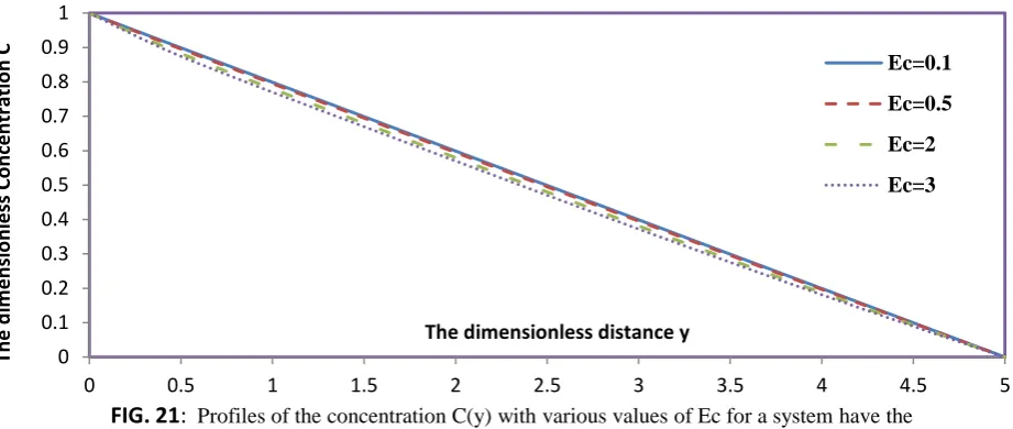
FIG. 21: Profiles of the concentration C(y) with various values of Ec for a system have the particulars =0.005, K=0.005, GT=2, Gc=4, Pr=0.7, Sr=0.2, Sc=5, J =0.2, 0.5π, c =3*106,

 =0.3, t0 =0.2

Ec=0.1

Ec=0.5

Ec=2