Testing of Rounded Corner for Micro-Drill on Hybrid of BP Neural Network and Adaptive Particle Swarm Optimization

(1)

Testing of Rounded Corner for Micro-Drill on

Hybrid of BP Neural Network and Adaptive

Particle Swarm Optimization

Wen-Jiang Xiang and Ying-Zhi Gu

Department of Mechanical and Energy Engineering, Shaoyang University, Shaoyang, P.R. China Email: [email protected], [email protected]

Dong-Yuan Ge

School of Mechanical and Automotive Engineering, South China University of Technology, Guangzhou, P.R. China Email: [email protected]

Abstract—A new approach based on hybrid of linear BP neural network and particle swarm optimization algorithm for fitting of micro-drill’s margin projection is proposed. The network is structured according to fitting equation, where sampled point coordinates of micro-drill and their recombination are taken as 6 inputs, and one output is obtained. The square of difference between the output and constant 0 is taken as performance index. The weights between input neurons and output neuron are tuned in the light of gradient descent method. In order to obtain global optimal solution, improved particle swarm optimization algorithm is integrated into the fitting program, where inertia weigh

ω

is modifying adaptively and mutation operator is carried on to increase the variety of particle dynamically. While the iteration is finish and the desired performance index of BP neural network is reached, thus stable weight values are obtained, according to which expression coefficients of ellipse can be solved. The rounded corner and diameter of the micro-drill can be tested easily. The presented approach provides a new solving method for ellipse fitting with advantages of programming easily and high precision.

Index Terms—BP neural network; particle swarm optimization; micro-drill; margin projection; rounded corner

I. INTRODUCTION

Micro-drill is applied in printed circuit board manufacturing industry widely, and its defects often take place in edge of cutting facet; if defects such as eccentric, rounded corner, main lips’ straightness errors (that is chips) are out-of-tolerance, they would result in vibration, excursion and break at super high speed processing, and decrease processing precision of PCB’s hole, such as hole wall surface roughness. The micro-drill’s defects should are smaller than 0.5

μ

m as for micro-drill’s diameter

among 0.1-0.3 mm [1-3]_{. There are many means such as} least squares method for ellipse or straightness fittingin the data processing [4]_{. By hybriding BP neural network} and particle swarm optimization algorithm, we put forward a novel data processing method to achieve the fitting of micro-drill’s margin projection and testing of its rounded corner and so on.

II. COLLECTION OF TRAINING SAMPLES

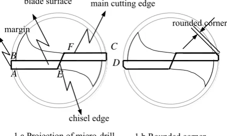
The projection of micro-drill blade surface is shown in Figure 1. Because the rounded corners locate at outermost of main lips, their linear speed are the highest, where the serious wear-out take place usually, and breaking and breach are inclined to resulting because of stress concentration. The rounded corner has large effect for the quality of micro-drill. While the rounded corners are measured, the steps are adopted as follows: measurement positions are the intersection points A and C that margin projection cuts across main cutting edges AE and FC.

Distances from A and C to actual edge of micro-drill are taken as rounded corner. Thus the key technique is to fit ellipse equation for the margin projection, and then the intersection points’ coordinates for A and C are acquired.

Fig.1 Projection of Micro-Drill

main cutting edge

chisel edge margin

blade surface

rounded corner

1.a Projection of micro-drill 1.b Rounded corner Figure 1. Blade surface of micro-drill A

B C

D E

F

(2)

Let the fitted equation of a micro-drill’s margin projection be as follows

0

2

2 ₊_bxy₊_cy ₊_dx₊_ey₊ _f ₌

ax ; (1)

where _a2 ₊_b2₊_c2₊_d2 ₊_e2 ₊ _f2 ₌1_.

III. FITTING OF MICRO-DRILL’S MARGIN PROJECTION

A. Linear BP Neural Network Structure

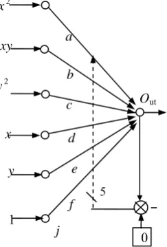
A BP neural network is designed to fit a micro-drill margin projection according to Eq. (1), whose structure is shown in Figure 2. The network’s input layer has 6 neurons, whose input signals are composed of sampled point coordinates, whose output lay has 1 neuron, its desired value is constant 0. The weights between input layer and output layer constitute a

vector _[ _]T

f e d c b

a，，，，， , whose elements are corresponding with the ellipse’s fitting coefficients in Eq.(1).

The input of the output neuron is

∑

= j

j T

net W I

,

j

=

1 ,

2 ,

"

,

6 .

(2)

where weight vectorW =

[

a，b，c，d，e，f

]

T , and

input vector T

I =[x2，xy，y2，x，y，1] .

The activation function f(x) is a linear function in the network, that is

f(x) =x+

_θ

.

(3) where

θ

is threshold, which is 0 in this experiment. The neuron’s output is shown as follows,

O= f(net)

.

(4)

During the learning, the square of difference between network’s actual outputs and desired value constant 0 is taken as performance index, which is shown as follows

₍ ₎2

2 1

O

E= −

.

(5) And the performance index is taken as objective functions for particle swarm optimization.

While the neural network is trained, the 6 weights

f e d c b

a, , , , , are tuned via errors back propagating in light of gradient descent rule. Thus the weights are tuned as follows [5-6]

)) 1 ( ) ( ( )

1

( + =− + − −

Δwj n

α

OIj

β

wj n wj n

,

(6)

where

α

>0 is learning rate;

β

>0 is momentum factor.

j

=

1 ,

2 ,

"

,

5 , t

he weights are iterated as follows

) ( ) ( ) 1

(n w n w n

wj + = j +Δ j

j=1,2,",5

.

(7) On the other hand, the 6th element is tuned as follows

⎪ ⎪ ⎩ ⎪⎪ ⎨ ⎧

< + + + +

− − − − − ± =

else ran

e d c b a

e d c b a f

(.)

1 1

2 2 2 2 2

. (8)

where ran(.)∈(-1,1) is random variable, while 1

2 2 2 2

2₊_b ₊_c ₊_d ₊_e _<

a , positive or negative is

selected for f in the light of its corresponding performance index being smaller.

B. Integration with Particle Swarm Optimization Algorithm

While the ellipse equation of micro-drill’s margin projection is fitted with BP neural network, its solution trajectory frequently trapped in local minima. In case the local minima, we integrate particle swarm optimization (PSO) algorithm to get out these minimum valleys, which is a stochastic optimization algorithm. In experiment swarm consists of 40 particles moving around in a 6 dimensional search space at a variant velocity according to individual experience and swarm experience adjusting their velocity dynamically, and the search space is(−1,1), each particle is taken as a potential solution to a problem. Assume the position of the ith_{particle is represented as}

) , , ,

( i1 i2 i6

i = x x " x

x ; the best previously encountered position of the ith_{particle is denoted its individual best} position pi =(pi1,pi2,",pi6), a value called pbesti; the best value of all individual pbesti values is denoted the global best positiongi =(gi1,gi2,",gi6) and called gbest; a velocity along each dimension is represented as

) , , ,

( i1 i2 i6

i = v v " v

v , the objective function is the

performance index of BP neural network, which is shown in Eq.(5). The updating equations are formulated as follows:

x xy

Out

1

5

j b a

c

0 2

x

2 y

y

d e

f

(3)

)) ( ) ( ( ) ( ( ) ( ) 1 ( 2 2 1 1 t t r c t r c t t i g i i i i x p x p v v − + − + =

+

ω

_.

₍₉₎

) 1 ( ) ( ) 1

(t+ = i t + i t+

i x v

x

.

(10)

where the velocity vector has three components, the first is the inertia which keeps the particle move next position, which plays the role of balancing the global and local searches, and coefficient

ω

has a bigger chance to find the global optimum within a reasonable number of iterations, a large inertia weight facilitates a global search while a small inertia weight favor high ability for local search; the second is the cognitive component, which is its own thoughts and experience; the third is the social component, which represents the messages shared all particle swarms and guide to the global best. c1 and c2 are the two acceleration coefficients, they are all set to values of 2.0 in the experiment; r1 and r2 are uniformly distributed in the range of [0, 1] [7-8]_.

C. Evolution speed factor and Square deviation of fitness

1. Evolution speed factor

The anti-evolution speed factor measures the performance of the particle evolution process of the PSO by far, it is expressed as follows,

1 1 )) 1 ( ( )) ( (

ε

+ − + = t g F t g F e best best

_.

(11)

where F(gbest(t)) is fitness value of current global optimum value;

ε

1 is constant nearly approximately zero

taken as offset bias value, in case F(gbest(t)) nearly equal to zero, and 0_≤e_<1. The larger the e is, the slower the evolution speed is; while e₌1, the algorithm stagnate or the optimal solving is achieved [9]_.

2. Square deviation of fitness

The square deviation of fitness describe the particles’ distribution, it is give by the following equation:

2 / 1 40 1 2 2

2, () }

) ( max{ )) ( ( 40 1 ⎥ ⎥ ⎦ ⎤ ⎢ ⎢ ⎣ ⎡ ⎟⎟ ⎠ ⎞ ⎜⎜ ⎝ ⎛ + − + − − =

∑

=

i g T T b

T i t F F F t F F t F ε ε

σ x .

(12)

where 40 is the number of population, F(xi(t)) denote the fitness of ith particle vector in tth iteration. Fb(t) is

the smallest fitness of particles, Fg(t) is the largest fitness of particles,

ε

2 is offset bias value which is

constant nearly approximately zero in case )

( ) (t F t

Fg − T

=0 or

FT(t)−Fb(t)

=0.

FT(t) is the mean value of current all particles’ fitness value in tth

iteration, that is

∑

= = 40 1 )) ( ( 40 1 i i

T F t

F x .

It is obvious that 0≤

σ

<1, and the bigger the σ

is

, the more diversity of particle is.

D. Self-adaptive algorithm of inertia weight

If the evolution speed of particle is fast, the algorithm can search optimization solving at large scope, if its evolution speed is slow, we can search at small space. On the other hand, if the square deviation of fitness of particle is small, the particle swarm will trap into local optimization, so we should improve dynamically the search space to improve the global optimization ability of particle. Thus according to the characteristic of the inertia weight

ω

[10-11]_{, which should increase along with the} increasing of gathering of particle, and decrease with decreasing of particle evolution speed accordingly, the dynamically modifying of inertia weight was proposed as follows,

σ

ω

= ini − e×e− σ ×

.

(13)

where ωini is the initial inertia weight, ωe

and

ω

σ are the coefficient of evolution speed factor and the square deviation of fitness; the range for them are defined as

1

0<

ω

e< , 0<

ω

σ <1.

E. Mutation mechanics of algorithm

On the other hand, a mutation operator is used by the view of genetic algorithm, which is the random-perturbation is adopted, the mutation coefficient is obtained as follows

⎩ ⎨

⎧ < >

= other f gBest andF k

pm d d

, 0

(

,

_σ

. (14)

where k is the any value between 0.1 and 0.2, 08

. 0

= d

σ

, fd =0.06.

The velocity mutation and position mutation are dealed with as follows

) 1 )( ( ) 1

(t v t r1

vij + = ij +

,

(15)

⎪ ⎪ ⎩ ⎪ ⎪ ⎨ ⎧ ≤ ≤ − − < ≤ − + = + 1 5 . 0 )) ( ) ( ( ) ( 5 . 0 0 )) ( ) ( ( ) ( ) 1 ( 2 min 2 2 max 2 r t x t x r t x r t x t x r t x t x ik ik ik ik ik ik

ik . (16)

where vij is the jth element of speed vector vi of ith particle selected according to pm, and xik is the kth element of position vector xi of ith particle selected according to pm, xikmax and xikmin are the boundaries of

position mutation element, that are -1 and 1; r1 and r2

are random between (0, 1).

IV. FITTING EXPERIMENT

(4)

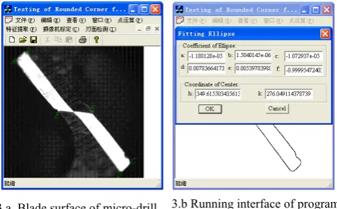
micro-drill is used to test in the experiment. Firstly its projection image is collected by CCD. While the projection of micro-drill margin is fitted, the sampled point’s coordinates should be obtained first. Then the corresponding 2D coordinates in image plane are estimated in the light of improved Canny operator and come to sub-pixel accuracy [12]_{. The projection of} micro-drill’s blade surface and running interface of program are shown in Figure 3.

In the program, let learning rate

α

=1×10−4 , and momentum factor

β

=1×10−5 , while the iteration is proceeded, and the iterations of BP neural network is 10 each generation interior; iterations of PSW is 280 generations; initial value of the network is generated at random, ωini =1.1, ωe =0.5, ωσ=0.04 , k=0.1, the offset value

ε

1=1×10−8,

ε

2 =1×10−8, As the training

is completed, that is the system comes to the global optimal point, thus the fitting equation of micro-drill margin projection was achieved according to the stable weights of BP neural network, which is shown follows,

2 5 6

2

5 ₁_.₅₀₄₀ ₁₀ ₁_.₀₇₂₉ ₁₀

10 1801 .

1 × − x − × − xy+ × − y

0 99995 . 0 10 3978 . 5 10 8366 .

7 3 3

= +

× −

×

− − _x − _y _{. (17)}

On the other hand, the equations of main cutting edge are obtained according to the proposed method as follows:

-1.74904×10−2 x +1.39356×10−2 y+0.99975 =0, (18)

-4.65656×10−3x +3.60398×10−3y +0.99998= 1. (19)

The centre of fitting ellipse O(h,k) can be solved according to Eq.(20),

2

2 ₄

2 ,

4 2

b ac

ae bd k b ac

cd be h

− − = −

−

=

.

(20)

Thus the centre (h, k) of ellipse is (349.6155, 276.0491) (measured in pixel). positions of measured that is the intersection points A and C are obtained

respectively. Rounded corners are the distances from A and C to actual edge of micro-drill. That is the minimum distances between intersection points A/C and sampled point are the rounded corner of micro-drill, which are 7.7664 (pixel) and 8.3052 (pixel) locating at (106.1424, 61.4774) and (593.7925, 489.7503) respectively; and the micro-drill’s diameter is 652.2397 (pixel). In the light of calibration data of camera, the object is 52 mm in length and the scale factor is 0.4569 (

μ

m/pixel) while system is working. Thus the micro-drill’s radiuses of rounded corners are 3.5485

μ

mand 3.7947

μ

mseparately; and the diameter of micro-drill is 0.2980mm.

If the least square method is adopted, its fitting equation can be obtained as follows

+ ×

− ×

+ ×

−₁_.₂₀₈₂₁₀−5 2 ₂_.₀₉₆₃₁₀−6 ₁_.₀₉₉₀₁₀−5 2

y xy

x

1 10 3303 . 5 10 8738 .

7 _× −3_x₊ _× −3_y₌ _{. (21)}

And the fitting equations of main cutting edge are obtained according to the least square method as follow

1.72582×10−2

x -1.36138×10−2y = 1, (22)

4.66039×10−3x -3.60904×10−3y = 1. (23)

If Hopfield NN is adopted, its solution trajectory always moves toward energy-lost direction, but frequently trapped in local minima, according to method which is partially similar in report [13]_{, the fitting equation} of micro-drill margin projection is shown as follows

+ ×

− ×

−₁_.₅₂₆₉ ₁₀−5 2 ₈_.₆₉₆₁ ₁₀−6 ₁_.₃₇₇₅ ₁₀−5 2

y xy

x

1 10 5431 . 4 10 3000 .

8 _× −3_x₊ _× −3_y₌ _{. (24)}

And the fitting equations of main cutting edge are obtained in the light of Hopfield NN as follow

1.72582×10−2 x -1.36138×10−2 y = 1, (25)

4.66039×10−3 x -3.60904×10−3 y = 1. (26) On the other hand, if the particle swarm optimization isn’t introduced, micro-drill’s margin projection is fitted only by BP neural network; its solution trajectory frequently is trapped in local minima. According to the method in research reports [14-15]_{, a fitted equation of} hyperbolic curve is obtained as follow:

1.1463 ₁₀4 2

x

−

× -2.5626×10−4xy+9.6251

₁₀

5 2

y

−

×

-9.0123

×

10

−3

x

+3.6054×10−2y=1. (27)

Thus the ellipse center, rounded corner and diameter obtained according to above fitting equations are obtained in Table 1.

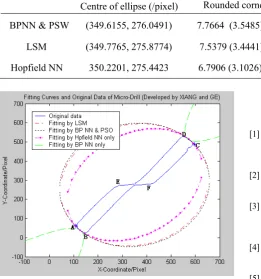
The original data and all fitting curves of the micro-drill according to Eq. (17), Eq. (21), Eq. (24) and Eq. (27) are shown in Figure 4.

Figure 3. Main interface of program

(5)

TABLE I. ELLIPSE CENTER AND TECHNOLOGY INDEXES OF MICRO-DRILL

Centre of ellipse (/pixel) Rounded corners /pixel (/μm) Diameter /pixel (/mm)

BPNN & PSW (349.6155, 276.0491) 7.7664 (3.5485), 8.3052 (3.7947) 652.2397 (0.2980)

LSM (349.7765, 275.8774) 7.5379 (3.4441),8.2385 (3.7642) 652.2314(0.2980)

Hopfield NN 350.2201, 275.4423 6.7906 (3.1026), 7.4456 (3.4019) 652. 2298 (0.2980)

V.CONCLUSION

The proposed approach has the following key features as opposed to other techniques: The coefficients of margin projection’s ellipse equation are obtained from the stable weight vector between the input layer and output layer of the BP neural network in the experiment. In order to obtain the global optimal solution, particle swarm optimization is integrated to fitting program, thus the coefficients of margin projection’s ellipse can be achieved. On the other hand, the characteristics of BP NN and Hopfield NN frequently trapped in local extremum is demonstrated in paper, too.

The proposed operator in this experiment possesses merits of programming easily and high accuracy, and makes the test system meet the precision requirement for intelligent test in many scenes, and has value of reference for data processing in machine vision and geometrical errors test of work-pieces.

ACKNOWLEDGMENT

The work is partially supported by National Hi-Tech Research and Development Program of China (2007AA04Z111), Scientific Research Fund of Hunan Provincial Education Department (07A062), Hunan Provincial Natural Science Foundation of China (09JJ6092), and Scientific Research Fund of Hunan Provincial Education Department (09B092).

REFERENCES

[1] F. C. Tien, C. H. Yeh, Hsieh K H. “Automated visual inspection for micro-drills in printed circuit board production”. International Journal of Production Research, 2004,vol 2, December 2004, pp. 2477-2495.

[2] S. L. HU. Machine Vision Based Precise Detection of PCB Micro-Drill’s Geometry Parameters [D]. Shanghai: Shanghai Jiao Tong University. 2009.9, pp. 27-43.

[3] S. L. HU, L. M. XU, K. Z. XU, et al.. “Adaptive Contour Corner Detection of Micro-drill’s First Facet ”. Journal of Shanghai Jiao Tong University. 2009,vol. 43, May 2009, 825-829.

[4] X.M. LI, S Z. Y. HI. “An Evaluation Method for the Roundness Error Based on Curvature”. Acta Metrologica Sinica, vol.29, April 2008, pp. 102-105.(In Chinese)

[5] J.Y, Chen, S.H. Chang, S.W.

Leu. “Adaptive BP neural network (ABPNN) based PN code acquisition system via recursive accumulator”. Proceedings of the 12th IEEE Workshop on Neural Networks for Signal Processing, 2002, pp. 737 - 745.

[6] X. F. Yao, Z. T. Lian, D. Y Ge, et al. “Approaches to Model and Control Nonlinear/Uncertain Systems by RBF Neural Networks”. International Journal of Innovative Computing, Information and Control, 2011, vol. 7, February 2011, pp. 941-954.

[7] Sheng Chen, Xia Hong, and Chris J. Harris. “Particle Swarm Optimization Aided Orthogonal Forward Regression for Unified Data Modeling”. IEEE TRANSACTIONS ON EVOLUTIONARY COMPUTATION, vol. 14, April 2010, pp. 477-499.

[8] H. C. Lee, S. K. Park, J.S. Choi, and B. H. Lee, “An Improved Fast SLAM Framework using Particle Swarm Optimization”]. Proceedings of the 2009 IEEE International Conference on Systems, Man, and Cybernetics, 2005, 3(2): pp. 211-216.

[9] X. P. ZHANG, Y. P. DU, G. Q. QIN, et al.. “Adaptive Particle Swarm Algorithm with Dynamically Changing Inertia Weight”, JOUNAL of XI’AN JIAOTONG UNIVERSITY, 2005, October 2005, pp.1039-1042.

[10]Wang L., X. T. Wang, J.Q Fu, L. L. Zhen. “A novel probability binary particle swarm optimization algorithm and its application”, Journal of Software, Vol.3, 2008, pp. 28-35.

[11]L. L. LIU, S. X. YANG, D. W. WANG. “Particle Swarm Optimization with Composite Particles in Dynamic Environment”. IEEE Trans. on Systems, Man, and Cybernetics-Part B: Cybernetics, vol.40, December 2010, pp. 1634-1648.

[12]J. Canny. A Computational Approach to Edge Detection [J]. IEEE. Transactions on Analysis and Machine Intelligence, vol. 8, June 1986, pp. 679-698.

(6)

[13]D.Y. GE, X. F.YAO and M. Q. YU. “Camera Calibration by Hopfield Neural Network and Simulated Annealing Algorithm”, ICIC-Express Letters, vol.4, August 2010, pp. 1257-1262.

[14]D. Y. GE, X. F. YAO, W. J. XIANG. Application of BP neural network for measurement of twist-drill circularity errors. Journal of Wuhan University of Science and Technology, vol. 32, August 2009, pp. 413-417. (In Chinese)

[15]W. J. XIANG, X. F. YAO, D. Y. GE. Application of BP Neural Network in Linear Fitting of Twist-Drill Main Lips. Machine Tool & Hydraulics, vol. 38, March 2010, pp. 21-24. (In Chinese)

Wen-Jiang Xiang, Shaoyang Hunan, 1963. Master, mechanical manufacture and its automation, Dongnan University, Nanjing, China. P. R. 1989; Ph.D candidate, mechanical manufacture and its automation, Hunan University, Changsha Hunan, China. P. R..

He is dean of teaching affairs office of Shaoyang University, there are 6 concerning previous published articles such as “Design and CAD system of the tool for drill flute”. Chinese Journal of Mechanical Engineering. December 2007, 20(6). His current and previous research interests are advance manufacture technology, precision manufacture and test, and intelligent optimization.

Pro. Xing was awarded a third award of science and technology progress of Hunan province, and a second award of science and technology progress of Shaoyang city.