FPGA Implementation Of DWT-SPIHT Algorithm
For Image Compression
I. Venkata Anjaneyulu, P. Rama Krishna
M. Tech Student, Department of Electronics & Communications, Anurag group of Institutions, A. P. India; Associate Professor of Electronics & communication Engineering, Anurag group of Institutions, A.P. India; Email: [email protected], [email protected]
Abstract: The main objective of the paper is to compress the image while transferring it from one end to the other, storage etc. This paper focuses on a memory efficient FPGA implementation for SPIHT (Set Partitioning in Hierarchical Trees) image compression technique. While compressing the image the wavelet transform converts the image into its wavelet coefficients. The SPIHTencoder receives the coefficient value and convert it into the bit stream. Then the SPIHT decoding and inverse wavelet transform will be performed to reconstruct the original image. Because of Poor image quality reconstruction, we are enhancing DCT to Discrete wavelet transform and EBCOT Encoding to SPIHT Encoding. These techniques are implemented on 2-D images and we can validate such compression algorithm by calculating PSNR (peak signal to noise ratio), MSE (Mean square error) and CR(Compression ratio). A hardware realization is done in a Xilinx 10.1 device and The improved algorithm keeps the high SNR, increases the speed greatly and reduces the size of the needed storage space.
Index terms: Image Compression, DWT, Spatial Orientation Trees, SPIHT.
I. INTRODUCTION
There are two types of image compression types and they are [1]Lossy compression [2]Lossless compression Lossy compression provides higher levels of data reduction but result in a less than perfect reproduction of the original image. It provides high compression ratio. Lossy image compression is useful in applications such as broadcast television, videoconferencing, and facsimile transmission, in which a some amount of error is an acceptable trade-off for increased compression performance. Lossless Image compression is the only acceptable amount of data reduction. It provides low compression ratio while compared to lossy. In Lossless Image compression techniques are composed of two relatively independent operations. (1) devising an alternative representation of the image in which its interpixel redundancies are reduced and (2) coding the representation to eliminate coding redundancies. Lossless Image compression is useful in applications such as medical imaginary, business documents and satellite images. There are many algorithms based on image compression. One of the most efficient algorithms is the Set Partitioning in Hierarchical Trees (SPIHT) algorithm1. This paper describes a MATLAB implementation of the SPIHT algorithm. Kai Liu [1] proposed a arithmetic architecture for SPIHT algorithm.This paper presented the pipelined architecture for DWT-SPIHT Algorithm.
II. WAVELET APPROACH
Storage constrains and bandwidth limitations in communication systems have necessitated the search for efficient image compression techniques. For real time video and multimedia applications where a reasonable approximation to the original signal can be tolerated, lossy compression is used. In the recent past, wavelet based image compression schemes have gained wide popularity. The characteristics of the wavelet transform provide compression results that outperform other transform techniques such as discrete cosine transform (DCT). Consequently, the JPEG2000 compression standard and FBI fingerprint compression system have adopted a wavelet approach to image compression. The wavelet coding techniques is based on the idea that the co-efficient of a
transform that decorrelates the pixels of an image can be coded more efficiently than the original pixels themselves. If the transform’s basis functions in this case wavelet- pack most of the important visual information into small number of co-efficient, the remaining co-efficient can be coarsely quantized or truncated to zero with little image distortion.
III. DISCRETE WAVELET TRANSFORMATION
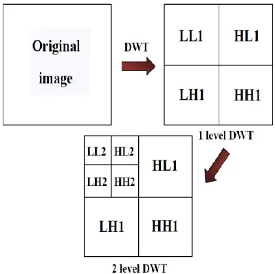
The second method of this mechanism uses 2-D Discrete Wavelet Transformation (DWT). DWT also converts the image from the spatial domain to frequency domain. According to the Fig. 1, the image is divided by vertical and horizontal lines and represents the first-order of DWT, and the image can be separated with four parts those are LL1, LH1, HL1 and HH1. In additional, those four parts are represented four frequency areas in the image. For the low-frequency domain LL1 is sensitively with human eyes. In the frequency domains LH1, HL1 and HH1 have more detail information more than frequency domain LL1.
A.1-D DISCRETE WAVELET TRANSFORM
The discrete wavelets transform (DWT), which convert a discrete time signal to discrete wavelet. The first step is to discretize the wavelet parameters, that reduce the continuous basis set of wavelets to a discrete and orthogonal / orthonormal set of basis wavelets.
m,n(t)=2 m/2
(2mt–n);m,nsuch that-< m,n <
The 1-D DWT is given as
Wm,n = < x(t), m,n(t) > ; m, n
ZThe 1-D inverse DWT is given as:
x (t) =
m n
n m n
m
t
W
,
,(
)
;m, n
ZB.2-D WAVELET TRANSFORM
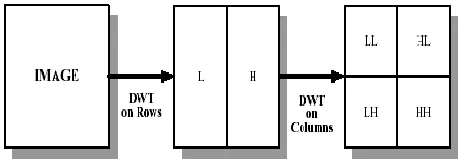
The 1-D DWT can be enhanced to 2-D transform using separable wavelet filters. By using separable filters, the 1-D transform to all the rows of the input and then repeating on all of the columns can process the 2-D transform. When one-stage 2-D DWT is applied to an image, four coefficient sets are created, and the sets are LL, HL, LH, and HH, Where L represents Low and H represents High.
Figure 2 Block Diagram of DWT (a) Original Image (b) Output image after the 1-D applied on Row input (c) Output
image after the second 1-D applied on row input
Figure 3 DWT for Lena image (a) Original Image (b) Output image after the 1-D applied on column input (c) Output
image after the second 1-D applied on row input
The Two-Dimensional DWT (2D-DWT) transforms images from spatial domain to frequency domain. At each stage of the wavelet decomposition, column of an image is first changed using a 1D vertical analysis filter-bank. The filter- bank is then applied horizontally to each row of the filtered and sub sampled data. One stage of wavelet decomposition produces four filtered and sub sampled images, called sub bands. The upper and lower areas of Fig. 3. (b), represent the low pass and high pass coefficients. The result of the
horizontal 1D-DWT and sub sampling to form a 2D-DWT output image is shown in Fig 3(c) We can use multiple levels of wavelet transforms to concentrate data energy in the lowest sampled bands. Specifically, the LL sub band in fig 2(c) can be transformed again to form LL1, HL1, LH1, and HH1 sub bands, producing a two-level wavelet transform. An (R-1) level wavelet decomposition is associated with R resolution levels numbered from 0 to (R-1), with 0 and (R-1) corresponding to the coarsest and finest resolutions. The forward convolution of 1D-DWT requires a large amount of memory and large computation complexity. Another implementation of the 1D-DWT, called lifting scheme, which give significant reduction in the memory and the computation complexity. The lifting approach computes the same coefficients as the direct filter-bank convolution.
IV.SPIHT
The SPIHT coder is a powerful image compression algorithm that produces an embedded bit stream from which the best reconstructed images in the mean square error sense can be extracted at various bit rates. The perceptual image quality, however, is not guaranteed to be optimal since the coder is not designed to explicitly consider the human visual system (HVS) characteristics.
Figure 4 SPIHT
Figure 5 Block Diagram
The image to be compressed is transformed into frequency domain using wavelet transform. In wavelet transform the images are divided into odd and even components and finally the image is divided into four levels of frequency components. The four frequency components are LL, LH, HL, HH, and then the image is encoded using SPIHT coding. Then the bit streams are obtained. The obtained are decoded using SPIHT decoding. Finally inverse wavelet transform is taken and the compressed image will be obtained.
SPIHT algorithm depends on 3 concepts: 1. Ordered bit plane progressive transmission 2. Set partitioning sorting algorithm
3. Spatial orientation trees.
Of these three concepts we are using Spatial Orientation Tree concepts in our thesis and the brief description of that is as follows,
V.SPATIAL ORIENTATION TREES
Normally, most of an image’s energy is concentrated in the low frequency components. Accordingly, the variance decreases as we move from the highest to the lowest levels of the subband pyramid. Moreover, it has been observed that there is a spatial self-similarity between sets, and the coefficients are expected to be better magnitude-ordered if we move downward in the pyramid following the same spatial orientation. For example, large low-activity areas are expected to be identified in the highest levels of the pyramid, and they are imitated in the lower levels at the same spatial locations. A tree structure, defines the spatial relationship on the hierarchical pyramid. Fig 6. shows how our spatial orientation tree is defined in a pyramid constructed with recursive four-subband splitting. Each node of the tree represents to a pixel and is identified by the pixel coordinate. Its direct descendants (offspring) correspond to the pixels of the same spatial orientation in the next finer level of the pyramid. The tree is defined as each node has either no offspring (the leaves) or four offspring, which always form a group of 2 x 2adjacent pixels. The pixels in the highest level of the pyramid are the tree roots and are also grouped in 2 x 2adjacent pixels. The following sets of coordinates are used to present the new coding method:
O (i, j): set of coordinates of all offspring of node (i, j); D (i, j) : set of coordinates of all descendants of the node
H: set of coordinates of all spatial orientation tree roots (nodes in the highest pyramid level);
L(i, j ) = D(i, j ) - O(i, j ) .
Figure 6 Spatial Orientation Tree
VI. IMPLEMENTATION IN FPGA
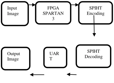
The below Block diagram shows the implementation of SPIHT image Compression in FPGA SPARTAN 3 kit.
Figure 7 FPGA Implementation
In this paper implementation of FPGA has four modules
Module 1: Conversion of image into Header file using GUI Module 2: Hardware Custom logic- EDK
Module 3: Micro blaze Processor design - EDK Module 4: Implementation in FPGA – EDK
A.CONVERSION OF IMAGE INTO HEADER FILE
Figure 8 Image Converted to a Header File
Using Matlab GUI, image file should be converted to a header file format. Then we add as an header file in our Impulse C code
B.HARDWARE CUSTOM LOGIC
Generating net list files and RTL schematic for the hardware peripherals used for SPIHT.
Generating bit file.
Input Image
SPIHT Decoding
SPIHT Encoding FPGA
SPARTAN 3
UAR T Output
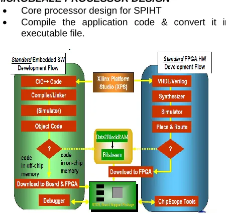
C.MICROBLAZE PROCESSOR DESIGN Core processor design for SPIHT
Compile the application code & convert it into executable file.
Figure 9 Diagram For Module 2& 3
XPS is part of the Xilinx Embedded Development Kit (EDK) and includes the Xilinx Platform Studio (XPS) GUI and all tools run by the GUI to process hardware and software system components. You can also perform system verification within the XPS environment
D.FPGA
Downloading bit file and executable file to FPGA through parallel interface.
Figure 10 FPGA Performance Advantage
VII.QUALITY MEASURES FOR IMAGE
The Quality of the reconstructed image is measured in terms of mean square error (MSE) and peak signal to noise ratio (PSNR) ratio. The MSE is often called reconstruction error variance q
2
. The MSE between the original image f and the reconstructed image g at decoder is defined as:
MSE=q 2
=
N
1
2
k j
k
j
g
k
j
f
,])
,
[
]
,
[
(
Where the sum over j, k denotes the sum over all pixels in the image and N is the number of pixels in each image. From that the peak signal-to-noise ratio is defined as the
ratio between signal variance and reconstruction error variance.
The PSNR value between two images having 8 bits per pixel in terms of decibels (dBs) is given by:
PSNR = 10 log10
MSE
2
255
When the PSNR value is 40 dB or greater, then the original and the reconstructed images are virtually indistinguishable by human eyes. The compression ratio of the image is given by
No of bits in original image
CR= --- No of bits in compressed image
The compression ratio shows that the image have been compressed.
Figure 11 SPIHT Algorithm With DWT Result
Table 1 PSNR Results In DB For Different SPIHT Coders
Image SPIHT-AC
SPIHT-NC
SPIHT-NL
SPIHT-HW
SPIHT-DWT
Lena
40.41
39.98
39.24
39.89
41.53
Airport
33.27
32.79
32.38
32.67
45.12
Woman
38.28
37.73
36.22
37.19
45.12
VIII.CONCLUSION
terms of speed can be achieved by introducing a lattice factorization of the wavelet kernel or by using the lifting steps.
REFERENCES
[1]. Kai Liu, Evgeniy Belyaev, and Jie Guo” VLSI Architecture of Arithmetic Coder Used in SPIHT” ieee transactions on very large scale integration (vlsi) systems, vol. 20, no. 4, April 2012
[2]. J.M. Shapiro, “Embedded image coding using zero trees of wavelet coefficients,” IEEE Trans. Signal Process., vol.41, no.12, pp.3445–3462, Dec. 1993.
[3]. Win-Bin HUANG, Alvin W.Y.SU“Vlsi implementation of a modified efficient spiht encoder” IEE TRANS. FUNDAMENTALS, VOL.E89–A, NO.12 DECEMBER 2006
[4]. A. Said, W. A. Pearlman “A new fast and efficient image codec based on set partitioning in hierarchical trees”IEEE TRANSACTIONS ON CIRCUITS AND SYSTEMS FOR VIDEO TECHNOLOGY, VOL. 6, PP 243 - 250, JUNE 1996.
[5]. K. K. Parhi, T. Nishitani “Vlsi architectures for discrete wavelet transforms “IEEE Transactions on VLSI Systems, pp 191 – 201,June 1993
[6]. T.W. Fry and S.A. Hauck “Spiht image compression on FPGAs” IEEE Trans. Circuits Syst. Video Technol., vol.15, no.9, pp.1138–1147, Sept. 2005”.
[7]. A. Aravind, M. R. Civanlar, and A. R. Reibman, “Packet loss resilience of MPEG-2 scalable video coding algorithms,” IEEE Trans. Circuits Syst. Video Technol., vol. 6, no. 5, pp. 426–435, Oct. 1996.
[8]. Y. Wang, G. Wen, S. Wenger, and A. K. Katsaggelos, “Review of error resilient techniques for video communications,” IEEE Signal Process. Mag., vol. 17, no. 7, pp. 61–82, Jul. 2000.
[9]. G. Cote, S. Shirani, and F. Kossentini, “Optimal mode selection and synchronization for robust video communications over error-prone networks,” IEEE J. Sel. Areas Commun., vol. 18, no. 5, pp. 952–965, Jun.2000.
[10]. S. Wenger, G. Knorr, J. Ott, and F. Kossentini, “Error resilience support in H.263+,” IEEE Trans. Circuits Syst. Video Technol., vol. 8, no. 7, pp. 867–877, Nov. 1998.
[11]. T. Wiegand, G. J. Sullivan, G. Bjontegaard, and A. Luthra, “Overview of the H.264/AVC video coding standard,” IEEE Trans. Circuits Syst Video Technol., vol. 13, no. 7, pp. 560–576, Jul. 2003.
[12]. P. Salama, N. B. Shroff, E. J. Coyle, and E. J. Delp, “Error concealment techniques for encoded video streams,” in Proc. Int. Conf. Image Processing, 1995, pp. 9–12.
[13]. Y. Wang and Q. F. Zhu, “Error control and concealment for video communication: A review,” Proc. IEEE, vol. 86, no. 5, pp. 974–997, May 1998.
AUTHORS PROFILES
.
I.Venkata Anjaneyulu, M. TECH (VLSI), CVSR College of Engineering, Ghatkesar, Hyderbad, A.P