Image DEnoising Method using Oli-Shrink, A
New Adaptive Wavelet Packet Thresholding
Function
Dhanusha. S. S Dr. Prof. M. Sasikumar
M. Tech Student Professor
Department of Electronics and Communication Engineering Department of Electronics and Communication Engineering
Marian Engineering College Marian Engineering College
Abstract
This paper proposes a statistically optimum adaptive wavelet packet (WP) thresholding function for image denoising based on the generalized Gaussian distribution. It applies computationally efficient multilevel WP decomposition to noisy images to obtain the best tree or optimal wavelet basis, utilizing Shannon entropy. It selects an adaptive threshold value which is level and subband dependent based on analyzing the statistical parameters of subband coefficients. In the utilized thresholding function, which is based on a maximum a posteriori estimate, the modified version of dominant coefficients was estimated by optimal linear interpolation between each coefficient and the mean value of the corresponding subband.
Keywords: Adaptive thresholding, image denoising, noise reduction, optimal wavelet basis (OWB)
________________________________________________________________________________________________________ I. INTRODUCTION
Efficient image denoising methods are still a challenge in the field of image processing. Most of the recently proposed denoising algorithms may work well in theoretical aspects but it will fail in practical applications. All show an outstanding performance when the image model corresponds to the algorithm assumptions but fail in general and create artifacts or remove fine structures and edges. Many denoising algorithm operate on the assumption that the noise level is known apriori, which in fact is not valid in practical circumstances. Image denoising is a technique used to improve the visualizing quality of the noisy image. The noisy image produces undesirable visual quality; it also lowers the visibility of low contrast objects. Hence noise removal is essential in digital imaging applications in order to enhance and recover fine details that are hidden in the data. The goal of denoising is to remove the noise while retaining as much as possible the important signal features.
Image denoising plays an important role in digital image processing. Image denoising is used to produce a good estimate of the original image from noisy image. There are so many kind of denoising process which provides the denoised image but the best procedure is which not only denoise the image but also remains its features like edges, contrast level etc. In image processing wavelet transform are widely used now a days. Wavelet has several advantages such as high degree of sparseness, excellent localization property etc. Image denoising involves the following three steps:
1) A linear forward wavelet transform; 2) Non-linear thresholding; and
3) A linear inverse wavelet transform.
In this paper a denoising technique which is based on wavelet packet transform is proposed. The wavelet packet method is a generalization of wavelet decomposition that offers a richer signal analysis. Wavelet packet atoms are waveforms indexed by three naturally interpreted parameters i.e. position, scale (as in wavelet decomposition), and frequency. For a given orthogonal wavelet function, we generate a library of bases called wavelet packet bases. Each of these bases offers a particular way of coding signals, preserving global energy, and reconstructing exact features. The wavelet packets can be used for numerous expansions of a given signal.
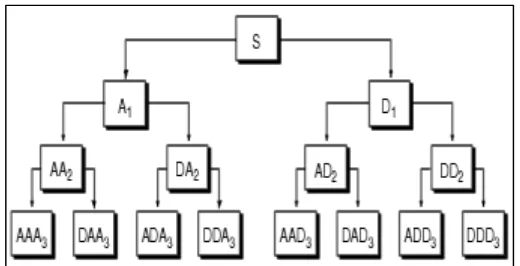
Fig. 1: Wavelet packet decomposition (in approximate A & detail part D of signal S)
In this paper, a statistical optimization process along with adaptive and subband-dependable methodologies are applied to both the thresholding function and wavelet transform, in order to advance the denoising even further. Unlike standard wavelet-based methods, we used WP transform (WPT) along with optimal wavelet basis (OWB) for image decomposition. Then, for each wavelet subband, an adaptive and subband dependent threshold value is calculated based on analyzing the subband’s statistical parameters. Next, a new thresholding function, called OLI-Shrink, is proposed to shrink small coefficients leading to calculate a modified version of dominant coefficients. The modification is done using optimal linear interpolation between each coefficient and the mean value of the corresponding subband. Compared with other prominent methods, the proposed algorithm has both significantly lowered the overall mean square error (MSE) and improved the visual appearance of the denoised image.
Fig. 2: Wavelet Packet Decomposition
II. RELATED WORKS
In the past three decades, a variety of denoising methods have been developed in the image processing and computer vision communities. Although seemingly very different, they all share the same property: to keep the meaningful edges and remove the less meaningful ones.
Image denoising is an open problem and has received considerable attention in the literature for several decades. Initially smoothing filters such as mean filter was used for denoising an image. Mean filter is an averaging linear filter. Here the filter computes the average value of the corrupted image in a pre-decided area. Then the center pixel intensity value is replaced by that average value. This process is repeated for all pixel values in the image. Though it serves as a simple technique it has the disadvantage of blurring the edges when reducing noise.
Order-Statistics filters are non-linear filters whose response depends on the ordering of pixel encompassed by the filter area. When the center value of the pixel in the image area is replaced by 100th percentile, the filter is called max-filter. On the other hand, if the same pixel value is replaced by 0th percentile, the filter is termed as min-filter.
Median filter is a best order static, non-linear filter, whose response is based on the ranking of pixel values contained in the filter region. Median filter is quite popular for reducing certain type of noise. Hence the center value of the pixel is replaced by the median of the pixel values under the filter region. Median filter is good for removing salt and pepper noise. These filters are widely used as smoothers for image processing, as well as in signal processing. A major advantage of median filter over linear filter is that the median filter can eliminate the effect of input noise values with extremely large magnitudes. Although the median filter can preserve edges, the fine structures are suppressed and it tends to produce regions of constant or nearly constant intensity in homogenous image regions.
Firstly similar image blocks are collected in groups. Blocks in each group are stacked together to form 3-D data arrays, which are de-correlated using an invertible 3D transform. The obtained 3-D group spectra are filtered by hard thresholding. The filtered spectra are inverted, providing estimates for each block in the group. These block-wise estimates are returned to their original positions and the final image reconstruction is calculated as weighted average of all the obtained block-wise estimates.
Many authors have developed image denoising algorithms based on statistical model of wavelet coefficients. For image modelling, a number of authors have developed models with hidden variables which control the local amplitudes of multiscale coefficients. The Hidden Markov Tree (HMT) models established Markovian parent-child relationships, hidden state variables rather than among the coefficient themselves. A local contextual Hidden Markov Model (HMM) offers an improvement and additional hidden variable is the local spatial activity, calculate as local average energy of the surrounding wavelet coefficients either across space, scale or orientation, additional improvement in denoising performance is obtained. The Gaussian Scale Mixture (GSM) model and its expansion in which clusters of coefficients are modeled as the product of Gaussian Random Vector and positive scaling variable, have been shown to produce results that are significantly better than HMM. Although the statistical model based method is popular and dominant in image denoising, it is hard to remove ringing artifacts of reconstruction. These methods tend to introduce additional edges or structures in the denoised image.
A non-linear iterative smoothing filter based on second order PDE is introduced which smoothen out the image according to an anisotropic diffusion process. Barbua et al. discussed a general variational model for image restoration based on the minimization of convex functional gradient under minimal growth conditions. This approach was related to minimization in bounded variation norm and has smoothing effect on degraded image, while preserving the edge features. Despite that they have obtained a better denoising effect, the anisotropic diffusion based image denoising tend to overblur the image and sharpen the boundary with many texture details lost.
The non-local methods estimate each and every pixel intensities based on information from the whole image, thereby exploiting the presence of similar patterns and features in an image. This relatively new class of denoising methods originates from the Non Local Means (NLM), introduced by Buades et al. Basically, the NLM filter estimates the noise-free pixel intensity as a weighted average of all pixel intensities in the image, and the weights are proportional to the similarity between the local neighborhood of the pixel being processed and local neighborhoods of surrounding pixels. Non local method has one limitation: both the objective quality and visual quality are inferior to other denoising techniques.
Without an explicit prior model on the signal, conditional random fields (CRF) are flexible at modeling short and long range constraints and statistics. Since the noisy input and clean image are well aligned at image features, CRFs can be well applied image denoising. However such an approach faces two challenges when applied to real world problems. First, the CRF’s energy function must be computationally feasible in the sense that minimum should be found in polynomial time. But, this does not usually happen in reality, since finding the global minimum for the most energy functions is Neymann Pearson (NP) hard. Second, it is very hard to find energy function that always have global minimum exactly at the desired solution.
A popular image denoising method is the bilateral filter where both space and angle distances are taken into account. The bilateral filter takes a weighted sum of the pixels in the local neighborhood; the weights depend on the both spatial distance and intensity distance. In this way edges are preserved while noise is averaged out. Bilateral filtering has been widely adopted as a simple algorithm for image denoising. However, it cannot handle speckle noise and it also has the tendency to over-smooth and to sharpen edges.
Fuzzy filters provide promising result in image-processing tasks that cope with some drawbacks of classical filters. Fuzzy filter is capable of dealing with vague and uncertain information. Sometimes it is required to recover a heavily noise corrupted image where a lot of uncertainties are present in this case fuzzy set theory is very useful. Each pixel in the image is represented by a membership function and different types of fuzzy rules that considers the neighborhood information or other information to eliminate filter removes the noise with blurry edges but fuzzy filters perform both the edge preservation and smoothing.
Using transform based methods, first step we transform image data to frequency or time –frequency domain using DFT and wavelet respectively, then keep only some large coefficients using the proper thresholding level and throw away rest. The small number of largest coefficients that has main information of image is kept and most noise coefficients that are small are set to zero. When we reconstruct the image from these coefficients, the noise has been reduced. However, if the noise or image’s parameters change, the thresholding level and our algorithms must be amended.
Wavelet Packet DE noising Algorithm Based on Correctional Wiener Filtering:
In this paper, in order to improve the quality of the degraded images, based on wavelet threshold denoising algorithm put forward by Donoho, the theory of Wiener filtering is analyzed and a denoising method using wavelet packet transforms based on the Wiener filtering is proposed. Firstly, the noisy
Image is processed by the correctional Wiener filtering and the noise standard deviation is calculated by the remaining signal of Wiener filter to regard as the threshold of wavelet packet transforms. Then the image is decomposed into the low frequency part and high frequency part by using wavelet packet transform and the wavelet packet tree coefficients are processed with soft threshold by using the level dependent adaptive threshold. Finally, the denoising image is acquired by using wavelet packet inverse transform.
DE noising of an Image Using Discrete Stationary Wavelet Transform and Various Thresholding Techniques:
The problem of estimating an image that is corrupted by Additive White Gaussian Noise has been of interest for practical and theoretical reasons. Non-linear methods especially those based on wavelets have become popular due
to its advantages over linear methods. In this paper they had applied non-linear thresholding techniques in wavelet domain such as hard and soft thresholding, wavelet shrinkages such as
Visu-shrink (non- adaptive) and SURE, Bayes and Normal Shrink (adaptive), using Discrete Stationary Wavelet Transform (DSWT) for different wavelets, at different levels, to denoise an image and determine the best one out of them.
Edge-Preserving Wavelet Thresholding for Image Demising:
In this paper, it provides a general setting for wavelet based image denoising methods. The denoised image f is obtained by minimizing a functional, which is the sum of a data fidelity term and a regularization term that enforces a roughness penalty on the solution. The latter is usually defined as a sum of potentials, which are functions of a derivative of the image. It considers new potential functions, which allows preserving and restoring important image features, such as edges and smooth regions, during the wavelet denoising process. Since important edges are characterized by high gradient magnitude, an efficient edge preserving denoising method must reduce shrinkage at points where the magnitude of the gradients exceeds certain thresholds, while shrinking coefficients corresponding to small values of the gradient, that are probably due to noise. Thresholding based Wavelet packet Methods for
Doppler Ultrasound Signal DEnoising:
This paper presents a threshold based wavelet packet denoising method, which preserves useful high frequency components and offers higher signal-to-noise ratio (SNR) compared with straight forward wavelet based denoising methods. To improve the selection of the threshold they propose several algorithms which are adaptive in the sense of coefficients obtained from different decomposed levels using the characteristics of the wavelet transforms. Wavelet packet denoising methods are quite applicable in Doppler Ultrasound signals because they have comparatively high frequency components dependent on flow velocity.
A New Wavelet Packet Based Method for DE noising of Biological Signals.
This paper introduces a new thresholding filter for the purpose of thresholding in denoising of EEG signals using wavelet packets. The functioning of the filter is examined and compared with that of hard and soft filters by applying this filter in denoising of EEG signals corrupted with white Gaussian noise. From the results, it is found that the new filter works better than hard and soft filters in addition to contain their features.
III. METHODOLOGY
Wavelet Packet Transform (WPT) is now becoming an efficient tool for signal analysis. To denoise the image the wavelet packet transform is used and the proposed methodology is shown in given flow chart. When compared with the normal wavelet analysis, it has special abilities to achieve higher discrimination by analyzing the higher frequency domains of a signal. The frequency domains divided by the wavelet packet can be easily selected and classified according to the characteristics of the analyzed signal. So the wavelet packet is more suitable than wavelet in signal analysis and has much wider applications such as signal and image compression, denoising and speech coding. We preserve the edge of the image by applying the edge detection technique. First o f all we add different kind of noise in the color image. After that the image will be decomposed by wavelet packet technique where we have to set the level, entropy thresholding and other parameters. We plot the wavelet packet tree and image on different node. By finding the best node, we have to denoise the wavelet packet and then display the image. Then we have to calculate the different parameters like PSNR, MSE etc. in order to find the performance of proposed method.
The steps for image denoising using wavelet packet are described below.
1) Wavelet packet decomposition. Choose a kind of wavelet to decompose the image using wavelet packet after determining its decomposing layers.
2) Determine the optimal base of wavelet packet according a given standard of entropy.
4) Wavelet packet reconstruction. Do the wavelet packet reconstruction according to the coefficient of the wavelet packet decomposition and the coefficient which is processed by quantification.
Flow chart
WP and Basis Extraction
Wavelets are localized in both time and frequency domains. In the traditional 1-D DWT, as shown in Fig. 1, the original signal L0 is transformed into low resolution (Ls) and high-resolution (Hs) subbands. At each stage it could be decided to split only the Ls or Hs part. Splitting the high resolution part result in Wavelet packet transform. In this type of transform, the optimal representation basis of the input signal is selected by optimizing a function known as “cost function” in each subband. The cost functions may determine the cost value for each node and its children in the obtained full binary tree. The algorithm starts with computing the cost values from the deepest level nodes. If the sum of the cost values for two children nodes is lower than the cost value of their parent node, then the children are retained, otherwise, they are eliminated.This cost value computation process is recursively repeated up to the tree’s root. The result is a basis that has the least cost among all the possible bases in this tree, so-called bestbasis or optimal basis.
Some of the cost functions are 1-norm, Shannon entropy, log entropy etc. Here Shannon entropy cost function is computed. The Shannon entropy of coefficients of subband S is calculated as follows:
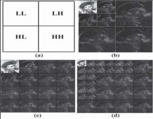
In this case, the original image is transformed into four pieces, which are normally labeled LL, LH, HL, and HH, as shown in Fig. 2(a). In this figure, both traditional DWT andWP decomposition used in our algorithm for selecting optimalwavelet basis are shown.
Fig. 3: Results of different wavelet decompositions. (a) Image decomposition scheme. (b) Traditional DWT. (c) WP decomposition. (d) Obtained OWB
Proposed Wavelet Shrinking Algorithm
In order to improve the denoising efficiency, a new adaptive thresholding function is introduced in this paper. Here an optimal wavelet basis is introduced for input image decomposition. The reason behind selecting the OWB packet is its dynamic decomposition nature in forming the subbands.
The threshold value is then picked up based on analyzing the statistical parameters of each subband coefficient. The thresholding function, necessary in the enhancement and/or elimination of the wavelet coefficients, is obtained using Bayesian maximum
aposteriori (MAP) estimate. Then, the optimal linear interpolation between each coefficient and the mean value of the corresponding subband are used to calculate the modified version of dominant coefficients.
Optimal wavelet basis
Algorithm for fast OWB extraction:
1) Choose L as the maximum number of levels for WP decomposition.
2) While the current level (d) of decomposition is less than L, for each existing subband (parent node) 𝑆𝑑𝑖(0≤ I <4𝑑− 1), do the following:
Compute the Shannon entropy as the cost function SE(𝑆𝑑𝑖)
Decompose𝑆𝑑𝑖 into four subbands (children nodes𝐿𝐿𝑑+14𝑖 ,𝐿𝐻𝑑+14𝑖+1,𝐻𝐿4𝑖+2𝑑+1, 𝐻𝐻𝑑+14𝑖+3) and compute the Shannon entropy of them: SE(𝐿𝐿4𝑖𝑑+1), SE(𝐿𝐻𝑑+14𝑖+1), SE(𝐻𝐿4𝑖+2𝑑+1), SE(𝐻𝐻𝑑+14𝑖+3)
If SE (𝑆𝑑𝑖) < (SE (𝐿𝐿4𝑖𝑑+1) + SE (𝐿𝐻𝑑+14𝑖+1) + SE (𝐻𝐿4𝑖+2𝑑+1) + SE (𝐻𝐻𝑑+14𝑖+3)), then only retain theparent node and eliminate children nodes, otherwise, retain parent and children nodes.
If there are no nodes to split, the process of extracting the OWB reaches the end.
Instead of the above highly computational complex algorithm, an alternative fast method for extracting OWB is employed. This method is a top-down search algorithm for selecting the optimal basis. The algorithm starts at the root and generates the optimal basis tree without growing the tree to full depth. In this algorithm, we use Shannon entropy to produce the optimal wavelet basis.
Threshold Selection Rules
In image denoising applications PSNR needs to be maximized, hence optimal value of threshold should be selected. Finding an optimal value for thresholding is not an easy task. If we select a smaller threshold then it will pass all the noisy coefficients and hence resultant images may still be noisy but larger threshold makes more number of coefficients to zero, which provides smoothness in image and image processing may cause blur and artifacts, and hence the resultant images may lose some signal values.
a) Universal Threshold
The universal threshold was proposed by Donoho and Johnstone as a global rule for one-dimensional signals. Regardless of the shrinkage function, for a signal of size n, with noise from a standard normal distribution N (0, 1), the threshold is:
b) Visu Shrink
Visu Shrink was introduced by Donoho. It follows hard threshold rule. The drawback of this shrinkage is that neither speckle noise can be removed nor MSE can be minimized. It can only deal with additive noise. Threshold T is given by
𝜆𝑢= 𝜎̂√2𝑙𝑜𝑔𝑛 (3) Where,
𝜎̂𝜂2= [𝑚𝑒𝑑𝑖𝑎𝑛(|𝑌𝑖,𝑗𝐻𝐻1|)
0.6745 ] 2
(4)
c) ayes Shrink
The BayesShrink rule uses a Bayesian mathematical framework for images to derive subband dependent thresholds that are nearly optimal for softthresholding. The formula for the threshold on a given subband s for the model given by the equation with zero mean variable X
𝑋𝑖,𝑗(t)=𝑆𝑖,𝑗(t)+𝜎𝜀𝑖,𝑗(t) , i=1,2,..I, j=1, 2,..J is given by,
𝜆𝑠= 𝜎 ̂^2
𝜎̂^2𝑠 (5)
Where 𝜎̂2 is the estimated noise variance and 𝜎 𝑠
̂2 is the estimated signal variance.
d) Proposed Method for threshold selection
In this algorithm, an adaptive threshold value λs for each subband S at level d is calculated as
𝜆𝑠= 𝛼𝑑,𝑠( 𝜎𝜂2
𝜎𝑋,𝑠) (6)
where 𝜎𝜂2 and 𝜎𝑋,𝑠2 are the variances of noise and clean image coefficients in the subband S, respectively. 𝛼𝑑,𝑠 is employed to make the threshold suitable in each decomposition level and each of subband. In other words, we set 𝛼𝑑,𝑠for a larger threshold values for high-frequency subbands based on their level of decomposition and their corresponding subbands.
The input noise variance is estimated by applying the robust median estimator on the HH1 subband’s coefficients
𝜎̂𝜂2= [𝑚𝑒𝑑𝑖𝑎𝑛(|𝑌𝑖,𝑗
𝐻𝐻1|)
0.6745 ] 2
(7)
Since the noise is additive, the observation model can be written as below
𝑌𝑖,𝑗𝑆 = 𝑋𝑖,𝑗𝑆 + 𝜂𝑖,𝑗𝑆 (8)
Where 𝑌𝑖,𝑗 𝑠 is the noise coefficients of subband S, 𝑋𝑖,𝑗𝑠 is the coefficients of the clean subband and𝜂𝑖,𝑗𝑠 is the noise coefficients. We assume that 𝑌𝑖,𝑗, 𝑋𝑖,𝑗 𝑎𝑛𝑑 𝜂𝑖,𝑗 have generalized Gaussian distribution models. Since the coefficients of the clean image and the noise are independent, we may write
σy,S2 = σx,s2 + ση2 (9) 𝜎𝑦,𝑠2 is the variance of coefficients (Yi, j ) in subband S. The value of 𝜎𝑋,𝑠2 , can be derived as
𝜎𝑥,𝑠2 = max ((𝜎𝑦,𝑠2 − 𝜎𝜂2), 0) (10)
𝛼𝑑,𝑠 is introduced to increase the threshold value in high-frequency subbands based on their level of decomposition and their positions at corresponding levels. A subband weighting function (SWF) in horizontal (𝑆𝑊𝐻𝐻) and vertical (𝑆𝑊𝐻𝑉) directions at level L of the WP decomposition is given by,
𝑆𝑊𝐹𝐻/𝑉(𝒊) = 𝑖2
22𝐿 for i = 1,2, … . . , 2
𝐿 (11)
Whereiis the index of subbands at the highest level of decomposition in horizontal and vertical directions, when decomposed subbands are arranged in the matrix structure. The value of 𝛼𝑑,𝑠 is given by,
αd,s= ∑ SWFH i∁s
(i) + ∑ SWFV(i) j∁S
(12)
Fig. 4: SWF used for computing the level and sub band-dependent threshold value
Thresholding Algorithm
Hard and soft thresholding techniques are used for purpose of image denoising. Keep and kill rule which is not only instinctively appealing but also introduces artifacts in the recovered images is the basis of hard thresholding whereas shrink and kill rule which shrinks the coefficients above the threshold in absolute value is the basis of soft thresholding. As soft thresholding gives more visually pleasant image and reduces the abrupt sharp changes that occurs in hard thresholding, therefore soft thresholding is preferred over hard thresholding.
In hard thresholding algorithm, the wavelet coefficients 𝑌𝑖,𝑗𝑠less than the threshold λs are replaced with zero. That is
𝛿𝜆𝐻𝑠(𝑌𝑖,𝑗𝑠) = {
0, |𝑌𝑖,𝑗𝑠| ≤ 𝜆𝑠 𝑌𝑖,𝑗𝑠, |𝑌𝑖,𝑗𝑠| > 𝜆𝑠
(13)
In the soft thresholding algorithm, however, the wavelet coefficients 𝑌𝑖,𝑗𝑠less than the threshold λs are replaced with zero and the others are modified by subtracting the threshold value λs using the following:
𝛿𝜆𝑠
𝑆(𝑌 𝑖,𝑗𝑠) = {
0 |𝑌𝑖,𝑗𝑠| ≤ 𝜆 𝑠 𝑠𝑖𝑔𝑛(𝑌𝑖,𝑗𝑠)(|𝑌𝑖,𝑗𝑠| − 𝜆𝑠) , |𝑌𝑖,𝑗𝑠| > 𝜆𝑠
(14)
In order to overcome the limitations of soft and hard thresholding a new algorithm called OLI-Shrink is introduced.
𝛿𝜆𝑠
𝑂𝐿𝐼(𝑌 𝑖,𝑗𝑠) = {
0 |𝑌𝑖,𝑗𝑠| ≤ 𝜆𝑠 𝑌𝑖,𝑗𝑠 − 𝛽(𝑌𝑖,𝑗𝑠 − 𝜇𝑠), |𝑌𝑖,𝑗𝑠| > 𝜆𝑠
(15)
Where 𝜇𝑠 is the mean value of the subband S, β is computed as follows:
𝛽 = 𝜎𝜂 2
(𝜎𝑋,𝑠2 + 𝜎𝜂2) ≅ 𝜎𝜂
2
𝜎𝑌,𝑠2
(16)
By using the Bayes rule, we can obtain the posterior probability density function (pdf) of x as below
𝑓𝑋 𝑌 ⁄ (𝑥 𝑦⁄ ) = 1 𝑓𝑌(𝑦) 𝑓𝑌 𝑋 ⁄ ( 𝑦 𝑥 ⁄ )𝑓𝑋(𝑥) 𝑓𝑋 𝑌 ⁄ (𝑥 𝑦⁄ ) = 1
𝑓𝑌(𝑦)𝑓𝜂(𝑦 − 𝑥)𝑓𝑋(𝑥) (17)
Where Y is the observed value and η is the additive white Gaussian noise. Since the wavelet coefficients in a subband of a natural image can be summarized adequately by a Gaussian distribution, we assume that x and η have Gaussian pdf
𝑓𝑋(𝑥) = 𝑁(𝑥, 𝜇𝑥, 𝜎𝑥2) = 1
√2𝜋𝜎𝑥𝑒𝑥𝑝 { −1 2𝜎𝑥2
(𝑥 − 𝜇𝑥)2}
𝑓𝜂(𝜂) = 𝑁(𝜂, 𝜇𝜂, 𝜎𝜂2) = 1 √2𝜋𝜎𝜂𝑒𝑥𝑝 {
−1
2𝜎𝜂2(𝜂 − 𝜇𝜂) 2
} (18)
Substitution of the pdf of x and η in (17) yields
𝑓𝑋 𝑌 ⁄ (𝑥 𝑦⁄ ) = 1 𝑓𝑌(𝑦) 1 √2𝜋𝜎𝜂𝑒𝑥𝑝 {
−1
2𝜎𝜂2(𝜂 − 𝜇𝜂) 2
} 1 √2𝜋𝜎𝑥𝑒𝑥𝑝 {
−1
2𝜎𝑥2(𝑥 − 𝜇𝑥)
𝑓𝑋 𝑌 ⁄ (𝑥 𝑦⁄ ) = 1 𝑓𝑌(𝑦) 1 2𝜋𝜎𝑥𝜎𝜂
𝑒𝑥𝑝 {−𝜎𝑥
2(𝑦 − 𝑥 − 𝜇
𝜂) − 𝜎𝜂2(𝑥 − 𝜇𝑥) 2𝜎𝑥2𝜎𝜂2
} (20)
To obtain the MAP estimate, we set the derivative of the log-likelihood function (ln(𝑓𝑥|𝑦(𝑥|𝑦)) with respect to x to zero as:
𝜕[ln(𝑓𝑋 𝑌
⁄ (𝑥 𝑦⁄ ))]
𝜕𝑥 =
2𝜎𝑥2(𝑦−𝑥−𝜇𝜂)−2𝜎𝜂2(𝑥−𝜇𝑥)
2𝜎𝑥2𝜎𝜂2 = 0 (21) From the above equation the MAP estimate is given by
𝑥̂ = 𝜎𝑋2
𝜎𝑋2+𝜎𝜂2(𝑦 − 𝜇𝜂) + 𝜎𝜂2
𝜎𝑋2+𝜎𝜂2𝜇𝑋 (22) The mean value of x is
𝜇𝑋= 𝜇𝑦− 𝜇𝜂= 1
𝑀𝑁∑ ∑ 𝑌𝑖,𝑗 𝑁
𝑗=1 𝑀
𝑖=1 (23) From (16) we can write,
𝜎𝑋2 (𝜎𝑋2+ 𝜎𝜂2)
= 1 − 𝜎𝜂 2
(𝜎𝑋2+ 𝜎 𝜂2)
= 1 − 𝛽 (24)
From weighted linear interpolation of the unconditional mean of x and the observed value y, x can be estimated.
𝑥̂ = 𝜎𝑋 2
𝜎𝑋2+ 𝜎 𝜂2
(𝑦 − 𝜇𝜂) + 𝜎𝜂 2
𝜎𝑋2+ 𝜎 𝜂2
𝜇𝑋
𝑥̂ = (1 − 𝛽)(𝑦 − 𝜇𝜂) + 𝛽𝜇𝑋
𝑥̂ = 𝑦 − 𝛽(𝑦 − 𝜇𝑦) (25)
This optimal linear interpolation between each coefficient and corresponding subband’s mean is combined with wavelet thresholding algorithm to yield the proposed thresholding function.
Algorithm of Denoising:
Step 1: Perform WP decomposition to obtain OWB of a noisy image by using Shannon entropy. Step 2: Estimate the noise variance
𝜎̂𝜂2= [
𝑚𝑒𝑑𝑖𝑎𝑛(|𝑌𝑖,𝑗𝐻𝐻1|) 0.6745 ]
2
Step 3: For each subband S in level d, compute the threshold value and statistical parameters: 1) The subband’s variance (𝜎𝑦,𝑠2 )
2) The subband’s mean (μs);
3) Estimate the variance of clean image using
σy,S2 = σx,s2 + ση2 4) The term 𝛼𝑑,𝑠 using
αd,s= ∑ SWFH i∁s
(i) + ∑ SWFV(i) j∁S
5) The term β using
𝛽 = 𝜎𝜂 2
(𝜎𝑋,𝑠2 + 𝜎𝜂2) ≅ 𝜎𝜂
2
𝜎𝑌,𝑠2 6) The threshold value using
𝜆𝑠= 𝛼𝑑,𝑠( 𝜎𝜂2 𝜎𝑋,𝑠
)
Step 4: Threshold all subband’s coefficients using the proposed thresholding technique given by
𝛿𝜆𝑂𝐿𝐼𝑠 (𝑌𝑖,𝑗𝑠) = {
0 |𝑌𝑖,𝑗𝑠| ≤ 𝜆𝑠 𝑌𝑖,𝑗𝑠 − 𝛽(𝑌𝑖,𝑗𝑠 − 𝜇𝑠), |𝑌𝑖,𝑗𝑠| > 𝜆𝑠 Step 5: Perform the inverse WPT to reconstruct the denoised image.
IV. EXPERIMENTAL RESULTS
The performance of the proposed noise reduction algorithm is measured using quantitative performance measures such as peak signal noise ratio (PSNR), MSE etc..
𝑃𝑆𝑁𝑅(𝑋, 𝑋̂) = 10 log10( 2552
𝑀𝑆𝐸) 𝑑𝐵 (26)
Where X is the original image and 𝑋̂is the denoised image and the MSE between the original and denoised images is given as
𝑀𝑆𝐸 = 1
𝑀𝑁∑ ∑ (𝑋(𝐼, 𝐽) − 𝑋̂(𝐼, 𝐽))) 2 𝑁
𝐽=1 𝑀
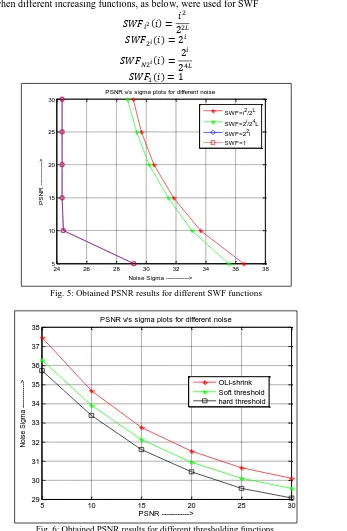
Where M and N are the width and height of the image, respectively. At first, to obtain a proper SWF, we evaluated the performance of the proposed method when different increasing functions, as below, were used for SWF
𝑆𝑊𝐹𝑖2(𝑖) = 𝑖2 22𝐿 𝑆𝑊𝐹2𝑖(𝑖) = 2𝑖
𝑆𝑊𝐹𝑁2𝑖(𝑖) =
2𝑖 24𝐿 𝑆𝑊𝐹1(𝑖) = 1
Fig. 5: Obtained PSNR results for different SWF functions
Fig. 6: Obtained PSNR results for different thresholding functions.
The results show that all SWF functions have good performance with the exception of function 𝑆𝑊𝐹 = 2𝐼. The proposed SWF shows slightly better performance. Next, the performance of the proposed thresholding function is evaluated by comparing it with the soft and hard thresholding methods. The obtained PSNR results for these thresholding functions are shown in Fig 6.
24 26 28 30 32 34 36 38
5 10 15 20 25 30
PSNR v/s sigma plots for different noise
P S N R - --->
Noise Sigma --->
SWF=i2/2L
SWF=2i/24L
SWF=22i
SWF=1
5 10 15 20 25 30
29 30 31 32 33 34 35 36 37 38
PSNR v/s sigma plots for different noise
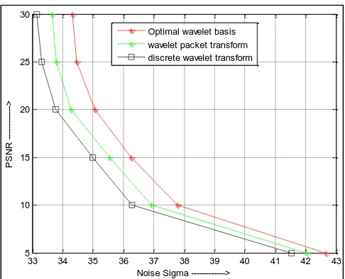
Fig. 7: Obtained PSNR results for various decomposition methods.
Fig. 7: Wavelet Packet decomposition for L=3
Fig. 8: Obtained Optimal Wavelet Basis
(a) (b)
33 34 35 36 37 38 39 40 41 42 43
5 10 15 20 25 30
P
S
N
R
-
--->
Noise Sigma ---> Optimal wavelet basis wavelet packet transform discrete wavelet transform
Tree Decomposition
(0,0)
(1,0) (1,1) (1,2) (1,3)
(2,0) (2,1) (2,2) (2,3) (2,4) (2,5) (2,6) (2,7) (2,8) (2,9) (2,10)(2,11)(2,12)(2,13)(2,14)(2,15)
(3,0) (3,1) (3,2) (3,3) (3,4) (3,5) (3,6) (3,7) (3,8) (3,9) (3,10)(3,11)(3,12)(3,13)(3,14)(3,15)(3,16)(3,17)(3,18)(3,19)(3,20)(3,21)(3,22)(3,23)(3,24)(3,25)(3,26)(3,27)(3,28)(3,29)(3,30)(3,31)(3,32)(3,33)(3,34)(3,35)(3,36)(3,37)(3,38)(3,39)(3,40)(3,41)(3,42)(3,43)(3,44)(3,45)(3,46)(3,47)(3,48)(3,49)(3,50)(3,51)(3,52)(3,53)(3,54)(3,55)(3,56)(3,57)(3,58)(3,59)(3,60)(3,61)(3,62)(3,63)
data for node: 0 or (0,0).
200 400 600 800 1000 1200
200
400
600
800
1000
1200
1400
Tree Decomposition
(0,0)
(1,0) (1,1) (1,2) (1,3)
(2,0) (2,1) (2,2) (2,3) (2,4) (2,5) (2,6) (2,7) (2,8) (2,9) (2,10)(2,11)(2,12)(2,13)(2,14)(2,15)
(3,0) (3,1) (3,2) (3,3) (3,4) (3,5) (3,6) (3,7) (3,8) (3,9) (3,10)(3,11)(3,12)(3,13)(3,14)(3,15)
(4,0) (4,1) (4,2) (4,3) (4,4) (4,5) (4,6) (4,7) (4,8) (4,9) (4,10)(4,11)(4,12)(4,13)(4,14)(4,15)
data for node: 0 or (0,0).
200 400 600 800 1000 1200
200
400
600
800
1000
1200
(a) (b)
(c) (d)
Fig. 8: (a) noisy image(noise variance-0.01), (b,c,d)-denoised image, (b)-OLI-Shrink, (c)-Soft Thresholding(d)-Hard thresholding noisy image-guassian
reconstructed-hard
reconstucted-soft
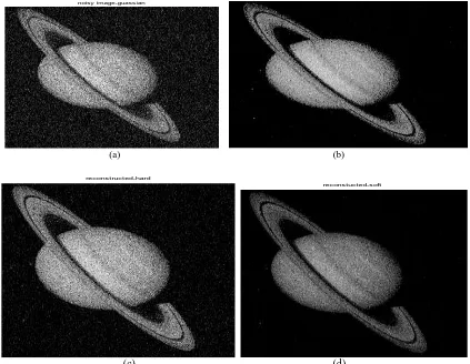
Fig. 9: (a) noisy image (standard deviation-10), (b,c,d)-denoised image, (b)-OLI-Shrink, (c)-Soft Thresholding(d)-Hard thresholding
(a) (b) (c) (d)
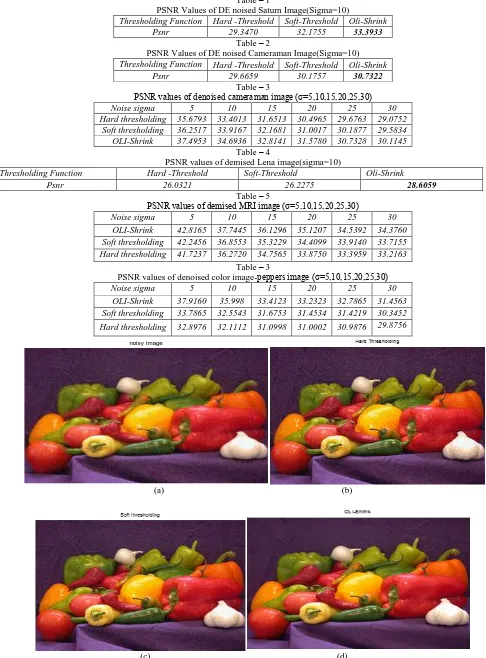
Fig 10-(a)-input image, (b) noisy image(noise variance=0.01), (c,d,e)-denoised image, (c)-Hard Thresholding,(d)-Soft Thresholding, (e)-OLI-Shrink
(a) (b)
(c) (d)
Fig. 11:(a) noisy MRI image (standard deviation-10), (b,c,d)-denoised image, (b)-OLI-Shrink, (c)-Soft Thresholding (d)-Hard thresholding
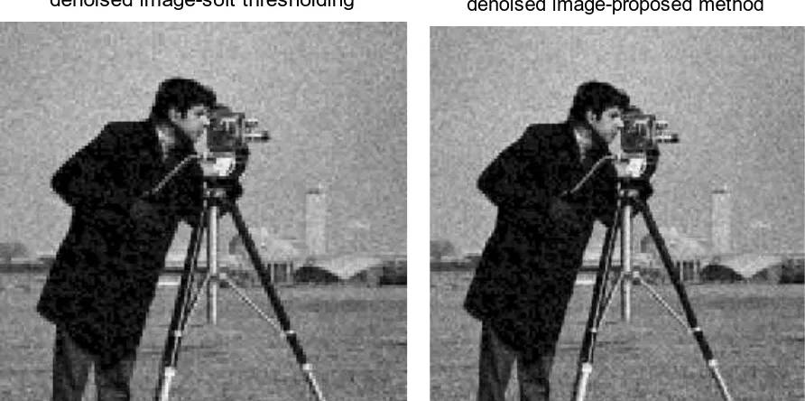
denoised image-soft thresholding
denoised image-proposed method
input image Soft thresholding
Table – 1
PSNR Values of DE noised Saturn Image(Sigma=10)
Thresholding Function Hard -Threshold Soft-Threshold Oli-Shrink
Psnr 29.3470 32.1755 33.3933
Table – 2
PSNR Values of DE noised Cameraman Image(Sigma=10) Thresholding Function Hard -Threshold Soft-Threshold Oli-Shrink
Psnr 29.6659 30.1757 30.7322
Table – 3
PSNR values of denoised cameraman image (σ=5,10,15,20,25,30)
Noise sigma 5 10 15 20 25 30
Hard thresholding 35.6793 33.4013 31.6513 30.4965 29.6763 29.0752 Soft thresholding 36.2517 33.9167 32.1681 31.0017 30.1877 29.5834 OLI-Shrink 37.4953 34.6936 32.8141 31.5780 30.7328 30.1145
Table – 4
PSNR values of demised Lena image(sigma=10)
Thresholding Function Hard -Threshold Soft-Threshold Oli-Shrink
Psnr 26.0321 26.2275 28.6059
Table – 5
PSNR values of demised MRI image (σ=5,10,15,20,25,30)
Noise sigma 5 10 15 20 25 30
OLI-Shrink 42.8165 37.7445 36.1296 35.1207 34.5392 34.3760 Soft thresholding 42.2456 36.8553 35.3229 34.4099 33.9140 33.7155 Hard thresholding 41.7237 36.2720 34.7565 33.8750 33.3959 33.2163
Table – 3
PSNR values of denoised color image-peppers image (σ=5,10,15,20,25,30)
Noise sigma 5 10 15 20 25 30
OLI-Shrink 37.9160 35.998 33.4123 33.2323 32.7865 31.4563 Soft thresholding 33.7865 32.5543 31.6753 31.4534 31.4219 30.3452
Hard thresholding 32.8976 32.1112 31.0998 31.0002 30.9876 29.8756
(a) (b)
(c) (d)
V. CONCLUSION
In this paper an efficient method for image denoising called OLI-Shrink is introduced. OLI-Shrink is compared with other thresholding methods such as hard and soft thresholding methods and it is found that the proposed method is better than other two methods. Also, the proposed method is applied on different set of images such as cameraman, Saturn, Lena, MRI image, Peppers etc. and OLI-Shrink provides denoised image with better PSNR and visually pleasing images than other methods. Image denoising using the proposed method excels in preserving the edge features of an image while reducing noise. Many denoising algorithms operate on the assumption that noise level is known apriori, which in fact is not valid in practical circumstances. The proposed method has achieved a high visual quality of the reconstructed image with minimum disturbing artifacts, while analytically ensuring the same in terms of quantitative metrics, with no information on the noise known apriori. The Proposed method is extended to color image also. The experimental results show the superiority of the proposed method over state-of-the-art denoising techniques. It can be further extended to video frame works.
REFERENCES
[1] D.L.Donoho, “Denoising by soft thresholding”, IEEE Trans. Inf theory, vol.41, may 1995
[2] Yunhong Li, Xin Yi, Jian Xu,“Wavelet packet denoising algorithm based on correctional Wiener Filtering ” Journal of Information & Computational Science
June 102013 pp 2711- 2718.
[3] Jiangfeng Yu, Dong C. Liu, “Thresholding based wavelet packet methods for Doppler ultrasound signal Denoiisng” IFMBE Vol. 19 2008 pp 408-412.
[4] V.V.K.D.V.Prasad, M. Suresh and A. Muralikrishna, “A New Wavelet Packet Based Method for Denoising of Biological Signals” International Journal of
Research in Computer and Communication Technology, Vol 2, Issue 10, October- 2013 pp 1056-1062.
[5] Abdullah Al Jumah, “ Denoising of an image using descrete stationary wavelet transform and various thresholding techniques ” Journal of Signal and Information Processing, 2013, 4, 33-41.
[6] D.Lazzaro,L.B.Montefusco,“Edge Preserving Wavelet Thresholding for Image Denoising” Journal of Computation and Applied Mathematics, 8 June 2006
pp222-231.
[7] Mantosh Biswas and Hari Om, “A new soft- thresholding image denoising method”,Elsevier,ICCCs-2012.
[8] Nezzamuddin Nezzamudini-Kachouie and Paul Ficguth, “Wavelet Packet Denoising Algorithm Based on Correctional Wiener Filtering”.IEEE tran. , CCECE,
MAY 2005.
[9] L.Sendur and I.W. Selesnick, ” Bivariate shrinkage functions for wavelet based denoising exploiting interscale dependency”, IEEE Trans. Signal Process.,