Multi-feature Fusion Face Recognition Based on
Kernel Discriminate Local Preserve Projection
Algorithm under Smart Environment
Di Wu1,2,31.College of Electrical and Information Engineering, Lanzhou University of Technology, Lanzhou,China 2.Key Laboratory of Gansu Advanced Control for Industrial Processes,Lanzhou,China
3.Manufacturing Engineering Technology Research Center of Gansu,Lanzhou,China
Email: [email protected]
Jie Cao1,2,3,4 , Jinhua Wang1,2,3,,Wei Li2,3,4
4. College of Computer and Communication, Lanzhou University of Technology, Lanzhou ,China
Email: {[email protected],[email protected], [email protected]}
Abstract—In this paper, a new face recognition method based on kernel discriminate local preserve projection(KDLPP) and Multi-feature fusion under smart environment is proposed . In order to solve the small sample size problem, combined with kernel theory and QR decomposition, a new face recognition algorithm named kernel discriminate local preserve projection is proposed based on discriminate local preserve projection algorithm. considered the external features are useful in face recognition, because hair is a highly variable feature of human face ,so we combined hair features and DCT features on the feature layer. The experiments on the AMI database indicate the proposed method can enhance the accuracy of the recognition system effectively.
Index Terms—Kernel Discriminate Local Preserve Projection(KDLPP), Hair Feature, Discrete Cosine Transform, Feature Fusion
I. INTRODUCTION
With the past decades , face recognition has become a very popular area of research in pattern recognition, computer vision and machine learning. Due to the immense application potential in military, commercial, building a automated system to recognize face in still images or video clips is necessary. Face recognition can be defined as the identification of individuals from images of their face by using a stored database of face labeled with people's identities[1]. This objective is very challenging and complex because the appearances of individual's face features are always affected by the factors such as illumination conditions, aging, 3D poses, facial expression and disguise including glasses and cosmetics[2]. Some other problematic factors such as noise and occlusion also impair the performance of the face recognition algorithms.
In the last ten years, face recognition under smart meeting room environment has been raised and become an hot research area. The smart meeting environment is installed four cameres on the four corner and microphone arrays on the table to tracking and
recognizing peoples joined in the meeting[3]. However, early studies all focused on the audio features and hardly any research based on visual features. Japanese researchers tried to use the visual characteristics of video sequence to study the communication process over the conference, they extracted the eye features between the people intercourse in the meeting, and using these features to present the influence degree of speaker to other peoples[4], to our best knowledge, this is the first time of researchers using visual features to discover the multi-people communication process, the drawback of this research is lack of quantitative analyse result of the experiment. In 2007, the research of IDIAP lab tried to use motion vector and residual encoding bit rate between two frames as face features[5]. In [6], chen used Discrete Cosine Transform coefficients as face features to recognize peoples in the meeting.
discriminant information in the null space of the locality preserving within-class scatter.
Most of the face recognition method mentioned above only use facial information, as we know, external information such as hair , facial contour and clothes also can provide the discriminant evidence[12]. Although external information are useful, but their detection ,representation, analysis and application are seldom been studied in the computer vision community. Ji et al.[13]used hair features for gender classification, they used length,area and texture infomation and split as hair features. Liu et al.[14]also used hair features for gender recognition.
In this paper, in order to solve the small sample size problem, by incorporating the kernel trick, a new face recognition algorithm based on discriminant locality preserving projections (DLPP) method and QR decomposition is proposed, which called kernel discriminant locality preserving projections (KDLPP) . The enhanced algorithm can not only handle the SSS problem,but also can adequate to describe the complex variation of face images. Considering the important role of hair features in face recognition, we study hair feature extraction and fusing with discrete cosine transform coefficient on the feature layer in order to capture the most recognize information.
The rest of this paper is organized as follows: in Section II we describe the feature extraction process of hair and face. Section III introduce the kernel discriminant locality preserving projections algorithm(KDLPP). We present our recognition method in Section IV. The experiment result are shown in Section V. Section VI offers our conclusion.
II. FEATUREEXTRACTION
A.Hair Feature Extraction
Hair is a highly variable feature of human appearance. It perhaps is the most variant aspect of human appearance. Until recently, hair features have been discarded in most of the face recognition system. To our best knowledge, their are two different algorithms in the literature about hair feature extraction. Yacoob et al.[15]developed a computational model for measuring hair appearance. They extracted several attributes of hair including color, volume, length, area, symmetry, split location and texture. These are organized as a hair feature vector. Lapedriza et al.[16] learned a model set composed by a representative set of image fragments corresponding to hair zones called building blocks set . The building blocks set is used to represent the unseen images as it is a set of puzzle pieces and the unseen image is reconstructed by covering it with the most similar fragments. We adopt the former method and modify it in this study.
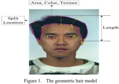
The basic symbols used in the geometric hair model are depicted in Figure 1. Here G is the middle point between the left point L and the right eye point R, I is the point on the inner contour, O is the point on the outer contour, and P is the lowest point of hair region.
Figure 1. The geometric hair model
The hair feature extraction consist of the following three steps:
1.Extract hair length features: we define the largest distance between a point on the outer contour and P as the hair length. The normalized distance
L
hair is defined as:face y
y
hair
dist
O
P
Girth
L
max(
(
,
))
/
(1)Where
Girth
face is the girth of the face region.2.Extract hair area features: we define the area covered by hair as the hair surface. Based on the hair model, the normalized hair area is defined as:
face hair
hair
alArea
alArea
Area
Re
Re
(2)Where
Re
alArea
hair is the real area of hair andface
alArea
Re
is the area of face.3.Extract hair color features: to obtain the color information in the hair region, we follow the method described in [17]. Based on this approach, the color distortion at pixel
i
is calculated byi i i
i
I
E
CD
(3)Where
I
i andE
i denote the actual and the expected RGB color at pixeli
respectively, theI
i isstated as follow:
))
(
),
(
),
(
(
I
i
I
i
I
i
I
i
r g b (4) According to the definition above, the color distortion at pixeli
is also can calculated as follows:2
2 2
)
)
(
(
)
)
(
(
)
)
(
(
b b i b
g g i g
r r i r
i
i
I
i
I
i
I
CD
(5)Where
i represent the current brightness with respect to the brightness of the model:2 2
2
2 2
2
)
(
)
(
)
(
)
)
(
(
)
)
(
(
)
)
(
(
b b
g g
r r
b b b g
g g r
r r
i
i
I
i
I
i
I
Where (
r,
g,
b ) and (
r,
g,
b )are the mean and standard deviation of color in the training set respectively. By use of equation (3),(5) and (6), we can obtain the expected RGB color values.)
,
,
(
E
rE
gE
bE
(7)By concatenating all the hair feature mentioned above, we obtain a feature vector of hair at pixel
i
asfollows: T i b i g i r hair hair i i
E
E
E
Area
L
color
area
length
Hair
]
,
,
,
[
]
,
,
[
,
(8)We normalized the hair region as size of
L
N
, sothe feature vector of hair region is represent as follow:
LN L N vectorHair
Hair
Hair
Hair
Hair
...
...
...
...
...
1 1 (9)B.Face Feature Extraction
We use discrete cosine transform(DCT) coefficients to characterize the face feature. DCT has been shown promising performance applied on the human recognition system.For an
M
N
image, where each imagecorresponds to a 2D matrix, DCT coefficients are calculated as follows[18]:
N v M u N v y M u x y x f v a u a v u C M x N y ,..., 1, 0 ,..., 1, 0 2 ) 1 2 ( cos 2 ) 1 2 ( cos ) , ( ) ( ) ( ) , ( 1 0 1 0
(10)Where
a
(
u
)
,a
(
v
)
is defined by :
otherwise
u
u
a
1
0
2
1
)
(
(11)
otherwise
v
v
a
1
0
2
1
)
(
(12))
,
(
x
y
f
is the image intensity function and)
,
(
u
v
C
is a 2D matrix of DCT coefficients.III. KERNELDISCRIMINANTLOCALPRESERVE PROJECTIONALGORITHM
A.Discriminant Local Preserve Projection Algorithm
A set of face image sample
{
x
i
}
can be representedas an
M
N
matrixX
[
x
1,
x
2,...,
x
N]
, whereM
is the number of pixels in the image and
N
is thenumber of samples. Each face image
x
i belong one of theC
face class{
X
1...
X
c}
. DLPP tries to maximize anobjective function as follows[19]:
C c c n j i T c j c i c ij c j c i C j i T j i ij j i y y W y y m m B m m1, 1 1 , ) ( ) ( ) ( ) ( (13)
Where
n
c is the number of samples in thecth
class, ci
y
represents theith
projected vector in thecth
class,
m
i andm
j is separately the mean of the projected vector for theith
class andjth
class, such as :
nik i k i i
y
n
m
1
1 (14)
njk j k j j
y
n
m
1
1 (15)Where
n
i andn
j is the number of samples in theith
class andjth
class separately.W
ijc represents theelements of within-class weight matrix and
B
ij represents the elements of between-class weight matrix:
exp(
2)
c j c i c ijx
x
W
(16))
exp(
2 2
j i ijf
f
B
(17) Where
is an empirically determined parameter, ci
x
represents theith
vector in thecth
class, andf
i isthe mean of the
ith
class:
nik i k i i
x
n
f
1
1 (18)Thus ,the between-class weight matrix
B
and thewithin-class weight matrix
W
are defined as follows:)
,...,
2
,
1
,
(
]
[
B
i
j
C
B
ij
(19))
,...,
2
,
1
,
(
]
[
jki ii
n
k
j
W
W
(20)Suppose that the mapping from
x
i toy
i isi T i
G
x
y
, then, the objective function (13) can berewritten as :
G
XLX
G
G
FHF
G
G
J
T T T T
)
(
(21)Where
L
andH
is Laplacian matrix and definedas follows:
W
D
L
(22)}
{
D
1,...,D
cdiag
D
(23)}
,...
{
1 cW
W
diag
B
E
H
(25)]
,...,
,
[
f
1f
2f
cF
(26)Where
D
i is a diagonal matrix and its elements are column sum ofW
i.E
also is a diagonal matrix and its elements are column sum ofB
.Now we should give the following definitions:
L T
w
XLX
S
(27)T L
b
FHF
S
(28)That the equation (21)can be rewritten as:
G
S
G
G
S
G
G
J
L w T L b T
)
(
(29)The transformation matrix
G
[
g
1,g
2,...,
g
k]
that maximize the objective function (29) can be obtained by solving the generalized eigenvalues problem:
k i L w i i L
b
g
S
g
g
g
g
S
,
1
1
...
(30)B. Kernel Discriminant Local Preserve Projection Algorithm
In this section , we present a new KDLPP algorithm to further improve the performance of DLPP algorithm.we using the kernel trick to handle the nonlinearity in a disciplined manner.The KDLPP algorithm involve two major steps[20]. The first step in to obtain the Gram matrix
K
and then to reduce thedimensionality of the original data features by applies the modified DLPP/QR algorithm.
The key idea of kernel Discriminant Local Preserve Projection Algorithm is to solve the problem of DLPP in an implicit feature space
F
, which is constructed by thekernel trick. Consider there is a feature mapping
which maps the input data into a higher dimensional inner product spaceF
[21]. So DLPP can be performedin
F
and it is equivalent to maximizing the following criterion:G
S
G
G
S
G
G
J
L w T L b T
)
(
(31)T L
w
X
L
X
S
(32)L T
b
F
H
F
S
(33)Referring to (31), any column of the solution
G
must lie in the span of all the samples in
F
, so there exitcoefficients
ij such that[22]:
c i i n j ij ijx
g
1 1)
(
(34)Where
g
represents any one column of theprojection matrix
G
. In other words, we can project eachvector onto an axis of
F
as follows:x t ij c i i n j ij
t x k x x
g
) , ( ) ( 1 1 (35) Where t c cn c n
x
(
k
(
x
11,
x
),...,
k
(
x
11,
x
),...,
k
(
x
1,
x
),...,
k
(
x
,
x
))
(36)t c cn c
ij
n
,...,
,...,
,...,
)
,...,
(
11
11
1
(37))
(
),
(
)
,
(
x
1x
2x
1x
2K
(38)Thus ,by using the definitions of L w
S
,S
bL and(35), we can obtain:
A
K
A
G
S
G
T bL
T bL (39)A
K
A
G
S
G
T wL
T wL (40) WhereT L
w
K
X
LK
X
K
(
)
(
)
(41)T L
b
K
F
HK
F
K
(
)
(
)
(42))]
(
),...,
(
),
(
[
)
(
X
K
x
1K
x
2K
x
NK
(43))]
(
),...,
(
),
(
[
)
(
F
K
f
1K
f
2K
f
CK
(44)N
i
x
x
k
x
x
k
x
x
k
x
x
k
x
K
t i c cn i c i n i i x i,...,
2,
1
))
,
(
),...,
,
(
),...,
,
(
),...,
,
(
(
)
(
1 1 1 11
(45)C
i
x
x
k
n
x
x
k
n
x
x
k
n
x
x
k
n
f
K
t i nk cnc ik i
i n
k c ik
i i n k i n
k n ik
i ik i i
,...,
2,
1
))
,
(
1
,...,
)
,
(
1
,...,
)
,
(
1
),...,
,
(
1
(
)
(
1 1 11 11 1 11
(46) So the objective of KDLPP can be written as follows:A
X
LK
X
K
A
A
F
HK
F
K
A
A
K
A
A
K
A
A
J
T T T T L w T L b T)
(
)
(
)
(
)
(
)
(
(47)Therefore , similar to DLPP algorithm, the optimal solution of equation (47) can be computed by finding the leading
r
eigenvalues{
i}
i1,2,...,r of(
K
wL)
1K
bLcorresponding to the nonzero eigenvalues. Once
]
,...,
,
[
1 1 rwe can map it to a
r
-dimensional space spanned by thecolumn of
A
. This projection is given byy
A
Tx
.The solution of
A
is complexly and always sufferfrom the small sample size problem, so we using QR decomposition matrix analysis to handle this issue[23,24]. The first step is to decompose L
b
K
as follows:T L b L b L
b
H
H
K
(
)
(48)Therefor we do QR decomposition on L b
H
byQR
H
bL
. for any given matrixG
R
rr, with)
(
Lb
H
rank
r
, the solution ofA
is given byQG
A
, thatG
k
G
G
k
G
QG
K
QG
QG
K
QG
A
J
w t
b t
L w t
L b t
~ ~
)
(
)
(
)
(
(49)
Q
K
Q
K
~b
t bL (50)Q
K
Q
K
~w
t wL (51) The final step is to compute an optimalG
bysolving the largest
r
eigenvalues problem on ~1 ~
)
(
K
w K
b . Table I resume the step of KDLPPalgorithm.
TABLE .I
PROCEDURE OF KDKPP ALGORITHM
Purpose: compute projection matrix
A
Steps:
1.compute
L
andH
from (22) and (25), thencompute
K
(
X
)
andK
(
F
)
from (43)and (44).2.Compute L w
K
andK
bL from (41) and (42).3.Construct
H
bL from equation (48).4.Perform QR decomposition on L b
H
,H
bL
QR
.5.Compute
K
~b
Q
tK
bLQ
,K
~w
Q
tK
wLQ
.6.Compute the
r
eigenvaluesg
i of~ 1 ~
)
(
K
w K
b , corresponding ther
largest eigenvalues.7.The projection matrix is
A
QG
with]
,...,
[
g
1,g
2g
rG
.IV. PROPOSED METHOD
In the past section we know how to extract hair features and DCT features, based on DLPP algorithm and kernel trick we give a new dimensional reduce technique called kernel discriminant local preserve projection algorithm. In this section , we give the face recognition algorithm based on multi-feature fusion and kernel discriminant local preserve projection algorithm. The main procedure of our method is depicted in Figure 2.
Training data
Hair feature extraction
DCT feature extraction
Feature fusion
Dimension reduction by KDLPP
Training feature
Testing data
Hair feature extraction
DCT feature extraction
Feature fusion
Dimension reduction by KDLPP
Testing feature
Recognition
Figure 2.Block diagram of recognition process
After extract the hair features and DCT features, we combined at feature-level as follows[25]:
]
[
TDCT T hair
fusion
F
F
F
(52)The steps of the training process is list as follows: (1) Extract the hair features and DCT features of the images in the training set .
(2) Fusing the hair feature and DCT feature at the feature level in order to obtain fusion feature.
(3) Analyse the fusion features in the training set utilizing the KDLPP algorithm to obtain the projection matrix
A
.(4) Project the training fusion feature into the lower dimensional space so that we can get the training features.
The steps of the recognizing process is list as follows:
(1) Extract the hair features and DCT features of the images in the test set.
(2) Fusing the hair feature and DCT feature at the feature level in order to obtain fusion feature.
(3) Project the test fusion feature into the lower dimensional space utilizing the projection matrix
A
which computed from training process.(4) classify the test set using the Minimum Euclidean Distance classifier.
V. EXPERIMENTS
A.AMI Database
“marketing director” for the task of designing a new remote control device. The teams met over several sessions of varying lengths (15–35 minutes).
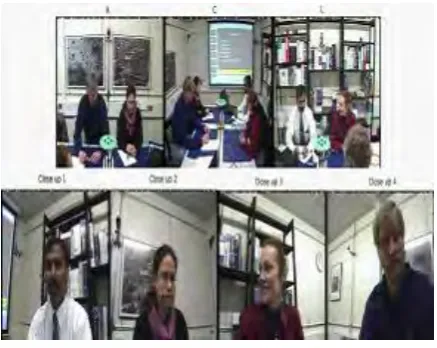
The meetings were not scripted and different activities were carried out such as presenting at a slide screen, explaining concepts on a whiteboard or discussing while sitting around a table. The participants therefore interacted naturally, including talking over each other. Data was collected in an instrumented meeting room. which contains a table, slide screen, white board and four chairs. While participants were requested to return to the same seat for the duration of a meeting session, they could move freely throughout the meeting. Different audio sources of varying distance to the speaker, and different video sources of varying views and fields-of-view represent audio-visual data of varying quality which is useful for robustness testing. Figure 3 show some samples captured form AMI database.
Figure 3.The captures of AMI database videos
In this experiment, the subset of AMI database named AMIES2016 was used . For this experiment, we captured 5 video segments from each people's video that at last a total of 20 small video segments were obtained. We denoted its as S1 to S20. For the reason of most of the image frames in the video have poor quality and no nose in the images, so we should delete it and then regular the image to guarantee nose is in the center of the image. Then select 10 frames from the video and record as 1 to 10 to construct the AMIES2016 face database. For each image, we normalized it to form the uniform size of 64*64. Figure 4 show 10 frames selected from one video.
Figure 4. Face images of AMIES2016 database videos
B.Experiment results
We randomly take
k
images from each class as thetraining data ,with
k
{
2
,
3
,...,
9
}
, and leave the restk
10
images as the test data. The Nearest Neighbour algorithm was employed using Euclidean distance for classification. There are three small experiments taken in our experiment as follows:Experiment A. Compare recognition accuracy based on KDLPP algorithm under different kernel functions.
The input data of the LDLPP is the kernel matrix and it is necessary to choose an adequate kernel function to construct this matrix. In this paper, we used Polynomial kernel function , Gaussian RBF kernel function and Fractional polynomial kernel function. Table II present the kernel functions used in our studies.
TABLE .II KERNEL FUNCTIONS
1.Polynomial kernel function
N
d
xy
y
x
K
(
,
)
(
1
d),
2.Gaussian RBF kernel function
)
2
exp(
)
,
(
x
y
x
y
2
2K
3.Fractional polynomial kernel function
1
0
),
1(
)
,
(
x
y
xy
d
K
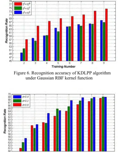
dIn order to illustrate the effect of kernel function choice, Figure 5 to Figure 7 show the results of KDLPP algorithm with different kernel functions. In Figure 5 we can show that for Polynomial kernel the performance decrease with the parameter
d
increasing. And globallygives less result than Gaussian RBF kernel function and Fractional polynomial kernel function. For Gaussian RBF kernel function, the value
2
10
9 gives maximum recognition rate compares to others values of
. The performance of Fractional polynomial kernel function with valued
0
.
4
is good but it is lower thanGaussian RBF kernel function.
Figure 5. Recognition accuracy of KDLPP algorithm
Figure 6. Recognition accuracy of KDLPP algorithm
under Gaussian RBF kernel function
Figure 7. Recognition accuracy of KDLPP algorithm
under Fractional Polynomial kernel function
Experiment B. Compare recognition accuracy based on different algorithms.
In this small experiment, we tested the FDA and DLPP methods compare to our proposed KDLPP algorithm, the kernel function used in this experiment is Gaussian RBF kernel function, the value
2
10
9 . Figure 8 give the recognition rate result. From the result we can show that KDLPP algorithm gives the best result under any training number situations, and FDA method give the worst result. From the figure we can also know that the face recognition rate under smart meeting environment is less than the standard face database environment because of the problem of poor quality image, lighting condition and facial expression change and so on.Figure 8. Recognition accuracy of different algorithms
based on hair and DCT feature fusion
Experiment C. Compare recognition accuracy based on KDLPP algorithm under different features.
In this small simulation, we compare the DCT feature with the hair and DCT feature fusion under KDLPP algorithm, the kernel function used in this experiment is Gaussian RBF kernel function, the value
9 2
10
, the recognition rate result are shown in Figure 9. From the result we can shown that hair feature play an important role in face recognition, the recognition result can improved significantly.Figure 9.Recognition accuracy of different features based
on KDLPP algorithm
VI. CONCLUSION
This paper investigate how to exploit effectively the hair feature information , as well as its fusion with face DCT feature for face recognition based on a new KDLPP algorithm under smart meeting room environment. The external information is crucial for face recognition, so we have presented a modified hair model for extracting hair features, by using this model, hair features are represented as length, area and color. In order to improve the accuracy we fusing it with the DCT features at the feature-level fusion for face recognition. SSS problem is always encountered by the DLPP algorithm, so we proposed a new KDLPP algorithm motivated by the idea of kernel trick and QR decomposition. By introducing a kernel function into discriminant criterion, KDLPP analyse the data in
F
and produces nonlineardiscriminating features that then can work on more realistic situations.
From the experiment result, we can obtain the following observations:(1) hair features play an important role in face recognition, (2) implementing the fusion of hair and DCT features can achieve the best classification accuracy in all of the case in face recognition, (3) KDLPP algorithm can handle the SSS problem and can work under more realistic situations.
ACKNOWLEDGE
This work was supported by the Science Foundation of Gansu Province,China (1010RJZA046). The Graduate Supervisor Foundation of Education Department of Gansu Province,China (0914ZTB003). The Finance
Department Foundation of Gansu
Province,China(0914ZTB148).
REFERENCES
[1] Cevikalp Hakan, Neamtu Marian, Wikes Mitch, Barkana Atalay. Discriminative common vectors for face recognition. IEEE Transactions on Pattern Analysis and Machine Intelligence 2005;27(1):4–13.
[2] Zhao W, Chellappa R, Phillips PJ, Rosenfeld A. Face recognition: a literature survey. ACM Computing Surveys 2003;35(4):399–458.
[3] Stergiou A, Pnevmatikakis A, Polymenakos L. The AIT Multimodal person identification system for CLEAR 2007. Multimodal Technologies for Perception of Humans, Lecture Notes in Computer Science, Baltimore, MD: Springer, 2008: 221-232.
[4] Carletta J, Ashby S, Bourban S, et al. The AMI meeting corpus: a preannouncement //In Proc of the Workshop on Machine Learning for Multimodal Interaction (MLMI). Edinburgh: 2005: 325-336.
[5] G.Garau and H.Bourlard. Using audio and visual cues for speaker diarisation initialisation. In Proc.International Conference on Acoustics,Speech and Signal Processing (ICASSP),2010:4942 - 4945.
[6] CHEN Yan-Xiang, LIU Ming.Audio-visual bimodal speaker identification in a smart environment[J].JOURNAL OF UNIVERSITY OF
SCIENCE AND TECHNOLOGY OF
CHINA.2010,40(5):486-490.
[7] X. He, S. Yan, Y. Hu, H. Zhang, Learning a locality preserving subspace for visual recognition, in: Proceedings of the Ninth International Conference on Computer Vision, France, October 2003, pp. 385– 392.
[8] X. He, S. Yan, Y. Hu, P. Niyogi, H. Zhang, Face recognition using Laplacian faces, IEEE Transactions on Pattern Analysis and Machine Intelligence 27 (3) (2005) 328–340.
[9] H. Hu, Orthogonal neighborhood preserving discriminant analysis for face recognition, Pattern Recognition 41 (2008) 2045–2054.
[10]W. Yu, X. Teng, C. Liu, Face recognition using discriminant locality preserving projections, Image Vision Computing 24 (2006) 239–248.
[11]L. Yang, W. Gong, X. Gu, W. Li, Y. Liang, Null space discriminant locality preserving projections for face recognition, Neurocomputing 71 (2008) 3644– 3649.
[12]S. Gutta, J.R.J. Huang, P.J., Wechsler, H.: Mixture of experts for classification of gender, ethnic,origin, and pose of human faces. IEEE Trans. Neural Networks 11(4) 948–960 (2000)
[13]Zheng Ji, Xiao-Chen Lian and Bao-Liang Lu. Gender Classification by Information Fusion of Hair and Face.Published by In-The. November 2008.
[14]LIU Shuang, X IE J in- rong, LU Bao- liang.Gender C lassification UsingHair Features.Journal of Computer Simulation. 2009:26(2),212-216.
[15]Yacoob, Y.: Detection and analysis of hair. IEEE Trans. Pattern Anal. Mach. Intell. 28(7)1164–1169 (2006)
[16]Member-Larry S. Davis.Lapedriza, A., Masip, D., Vitria, J.: Are external face features useful for automatic face classification? In: CVPR ’05: Proceedings of the 2005 IEEE Computer Society Conference on Computer Vision and Pattern Recognition (CVPR’05)
[17]Yacoob, Y., Davis, L.: Detection, analysis and matching of hair. The tenth IEEE International Conference on Computer Vision 1 741–748 (2005)
[18]Z M Hafed ,M D Levine. Face recognition using the discrete cosine transform.International Journal of Computer Vision ,2001 ,43 (3) :167 - 188.
[19]W. Yu, X. Teng, C. Liu, Face recognition using discriminant locality preserving projections, Image Vision Computing 24 (2006) 239–248.
[20]Baochang Zhang,Yu Qiao.Face recognition based on gradient gabor feature and Efficient Kernel Fisher analysis.Neural Computing & Applications,2010,19(4):617-623.
[21]Wen-Chung Kao, Ming-Chai Hsu, Yueh-Yiing Yang. Local contrast enhancement and adaptive feature extraction for illumination invariant face recognition.Pattern Recognition,2010,43(5): 1736-1747.
[22]PARK H,PARK C H. A comparison of generalized linear discriminant analysis algorithm.Pattern Recognition, 2008,41(3):1083-1097.
[23]Kazuhiro Hotta. Local normalized linear summation kernel for fast and robust recognition.Pattern Recognition, 2010, 43(3):906-913.
[24]MA Xiaohong,ZHAO Linlin.A robust audio watermarking method based on QR decomposition and lifting wavelet transform.Journal of Dalian University of Technology,2010,50(2):278-282
[25]Shufu Xie, Shiguang Shan, Xilin Chen, Jie Chen. Fusing Local Patterns of Gabor Magnitude and Phase for Face Recognition. IEEE TRANSACTIONS ON IMAGE PROCESSING, 2010,19(5):1349-1361.
[26] http://www.amiproject.org/.
recognition.
He joined in The Science Foundation of Gansu Province and The Graduate Supervisor Foundation of Education Department of Gansu Province. also he present some papers:"Face Recognition Based On Pulse Coupled Neural Network";"Combination of SVM and Score Normalization for Person Identification based on audio-visual feature fusion" and so on . all indexed by Engineering Index.
JIE CAO, born in October 1966, Suzhou, Anhui, China. JIE CAO received B.Tech. degree from Ganshu Institute of Technology in 1987, Lanzhou, China, and the M. Tech. degree from Xi’an Jiaotong University in 1994. Hers research interests lie in the areas of information fusion and Intelligent Transportation (ITS).
She is a professor of Lanzhou University of Technology, doctoral tutor, and the "second level" candidates of Gansu leading talent. She presided over the completion of the "Gelatin production process of integrated automation control systems and process parameters optimization," during 2007 to 2010, and got the second Award of Gansu Provincial Science and Technology Progress. She participate Canada and China inter-governmental cooperation project "Regional planning and transport system” of the Canadian International Development Agency (acceptance); organizated implementation of the National Technology Support Program "for the key industries of manufacturing information integration platform and application" by the Ministry of Science and acceptance; chaired or participated in 20 projects , currently hosted mainly in the research project are: Natural Science Foundation of Gansu Province, " visual detection, identification and tracking Research based on the sports car "; Gansu Higher operating costs of basic scientific research,"multi-speaker recognition based on audio and video feature fusion "; Natural Science Foundation of Gansu Province, " multi-Speaker Tracking based on the audio and video feature fusion ".
JINHUA WANG , born in Tianshui, Gansu province of China in 1978. Received B.Tech. degree from Xi’an university of science and technology in 2001,Xi’an, China, and the M.Tech. degree from Lanzhou university of technology in 2010. Her research interests lie in the areas of Information Fusion and Intelligent Transportation (ITS).
She is a Lecturer of Lanzhou University of Technology, and participated in 10 projects. She won first prize in science and technology progressof Gansu Province in 2010.Currently joined mainly in the research project are: Natural Science Foundation of Gansu Province, " visual detection, identification and tracking Research based on the sports car "; Gansu Higher operating costs of basic scientific research,"multi-speaker recognition based on audio and video feature fusion "; Natural Science Foundation of Gansu Province, " multi-Speaker Tracking based on the audio and video feature fusion ", ADB loan Lanzhou urban transport project advanced traffic control system (ATCS) project (design). Also she present some papers:"Research on moving vehicles tracking algorithm based on feature points and AKF", "A Object Tracking Algorithm Based on the Points of Feature Fusion","The maneuvering target tracking based on the improved "current" statistical model and AKF",and so on.