Multi-dimensional Time Series Approximation Using
Local Features at Thinned-out Keypoints
Yu Fang, Do Xuan Huy, Hung-Hsuan Huang, Kyoji Kawagoe*
Ritsumeikan University, Kusatsu, Shiga, Japan.* Corresponding author. email: [email protected]
Manuscript submitted August 1, 2014; accepted September 25, 2014. doi: 10.17706/jcp.10.1.1-11
Abstract: A multi-dimensional time-series is a sequence of vectors measured by many devices at points in time. Although many methods have been proposed to model and classify the data, these methods lead to a problematic relationship between cost and accuracy. In this paper, we propose a novel method for approximating multi-dimensional time-series, named multi-dimensional time-series Approximation with use of Local features at Thinned-out Keypoints (A-LTK), which enables an adequate accuracy value to be obtained even when reduced storage cost is a requirement. The main concepts of A-LTK are 1) reduction of time points and 2) construction of local features at the thinned-out keypoints. A preliminary evaluation indicated that with these points our proposed method was capable of achieving almost the same accuracy with less storage cost, compared to existing methods.
Key words: Multi-dimensions, times series, classification, approximation, keypoint extraction, local features.
1.
Introduction
Rapid progress in the development of sensor devices has resulted in sensors with the ability to continuously acquire multiple time series data. For example, motion capture systems can output multiple streams of observed stream data on each marker position [1]. The latest smartphones and tablets can measure geographical locations which means that data from multiple sensors equipped with mobile devices such as these can be used for activity estimations. Sensors are also useful for predicting extreme weather, for example, some parts of the world are repeatedly struck and damaged by heavy storms such as hurricanes, typhoons, or cyclones. Because predicting the track of a storm is important for preventing damage, data of the characteristics for storms is measured on a continuous basis [2]. The data, which is generated as multi-dimensional time-series, include the location, speed, direction, max-wind-velocity, low-atmospheric-pressure, force-win-radius of the storm.
Symbolic ApproXimation (SAX) [5] that is used to approximate each time series composing multi-dimensional data [6].
In this paper, we propose a novel method for approximating a multi-dimensional time series as one of the second category methods, the contour-based method. The new method, the Approximation with use of Local features at Thinned-out Keypoints (A-LTK), is proposed to introduce two basic ideas which are 1) reduction of time points and 2) construction of local features at the thinned-out keypoints. Owing to the use of these ideas, a multi-dimensional time-series can be approximated with smaller storage costs.
2.
Multi-dimensional Time Series
A multi-dimensional time-series is defined as a sequence of vectors, that is, TS = <v1, v2, ..., vn>, where vk is
a d-dimensional vector at a time tk. When k=1, TS is a time series of scalar values, that is one dimensional time series. For our purpose, the assumption is made that the length of TS, n, is a variable. A query Q is also defined as a sequence of d-dimensional vectors qk. Q=<q1,q2, ..., qm>.
Given a multi-dimensional time-series TS and a query Q, the similarity between TS and Q is defined as sim(TS, Q). There are several ways to realize the function sim(TS, Q). If the lengths of the two time series are the same, i.e. when n=m, the Euclidean can be used:
n
i d vi qi
Q TS sim 1 2 )) , ( ( /( 1 ) , ( ,
where
v
i andq
i are the i-th vectors of TS and Q at a time ti, respectively.)
,
(
v
iq
id
is a distance function which returns the distance betweenv
i andq
i. Distance measures like the Euclidean or the cosine distance can be used as the distance function d.Another way to determine the similarity is to use Dynamic Time Warping (DTW) [7]:
0 0 , 0 ) ,
(TS Q if n and m
DTW
0
0
,
)
,
(
TS
Q
if
n
or
m
DTW
otherwise Q Rest TS Rest DTW Q TS Rest DTW Q Rest TS DTW Q Head TS Head d Q TS DTW )) ( ), ( ( ), ), ( ( ), ( , ( min( )) ( ), ( ( ) , ( In the above definition, Head(A) is the first vector of A and Rest(A) is a sequence that remains after HEAD(A) is removed from A.
Moreover, Longest Common Subsequence (LCS) can be used to calculate the similarity between multiple time series [8]:
0 0 , 0 ) ,
(TS Q if n orm
LCS
m n and Q Head TS Head d if Q Rest TS Rest LCS Q TS LCS )) ( ), ( ( )) ( ), ( ( 1 ) , ( otherwise Q Rest TS LCS Q TS Rest LCS Q TS LCS )) ( , ( ), ), ( ( max( ) , ( In the definitions of both DTW and LCS, the distance between HEAD(A) and (Q) needs to be calculated for which either the cosine distance or Euclidean can be used.
Finally, the Edit distance can be applied to the distance between two multi-dimensional time series. The method is called Edit Distance on Real sequence (EDR) [9] and is defined as follows:
0
)
,
0
)
,
(
TS
Q
m
if
n
EDR
otherwise Q Rest TS EDR Q TS Rest EDR C Q Rest TS Rest EDR Q TS EDR ) 1 ) ( , ( , 1 ) ), ( ( , ) ( ), ( ( min( ) , ( Some extended methods have been proposed based on these basic methods. One example of the extensions is Angular Metric for Shape Similarity (AMSS) that is defined as follows [10], [11]:
In AMSS, the difference time series is first calculated from the original data. The difference A of the time
series
A
a
1,
a
2,...,
a
n
is defined as
A A1, A2,..., An1 ,
where Ak ak1akfor any k 1,...,n1 Then, 1 1 ) , ( ]) , 1 [ ], , 1 [
(TS i Q j Simv1 q1 ifi andj
S 1 1 ]) , 1 [ ], , 1 [
(TS i Q j ifi or i
S )) , ( ] , 1 [ ], 1 , 1 [ ( ), , ( ] 1 , 1 [ ], , 1 [ ( ), , ( ] 1 , 1 [ ], 1 , 1 [ ( max( ]) , 1 [ ], , 1 [ ( j i j i j i q v Sim j Q i TS S q v Sim j Q i TS S q v Sim j Q i TS S j Q i TS S ]) 1 , 1 [ ], 1 , 1 [ (( ) ,
(TS Q S TS n Q m
AMSS ,
where Sim(vi,qj)cos (viqj)/(vi,qj)
As shown in the above definition, AMSS determines the set of difference vector pairs producing the most similarity.
All of the above methods are processed for all the vectors of a sequence. In other words, vectors at all time-points are used to calculate time series similarities. Any of the methods, DTW, LCS, EDR and AMSS, is calculated by using a certain kind of dynamic programming scheme. Therefore, the cost of O(n2) is necessary to obtain a distance value where n is the number of time-points in the time series.
There are several methods, such as APCA [12] and SAX [5], could be used to reduce the cost in the single dimension time series, although a cost reduction method has not yet been developed for multi-dimensional time series. Therefore, in this paper, a novel method for approximating a multi-dimensional time series, called A-LTK, is proposed together with a technique that introduces thinned-out keypoints. This technique is capable of reducing the storage cost in A-LTK in addition to the computational cost. The basic principles of A-LTK are discussed in the next section.
SAX is a popular and effective method for approximating single-dimension time series. Several methods have been proposed that use SAX for approximating multi-dimensional time series. However, in this research, SAX is not considered an alternative for A-LTK, because it is a symbolic approximation method for of time series, whereas A-LTK is essentially a method approximated by reducing the number of time points. While SAX could also be implemented as a part of A-LTK, the latter method uses a local feature-based approximation instead of symbols.
PCA is not mentioned because it can easily employed before our method is used for processing, as a pre-processing step.
3.
Approximation
Using Local Features at Thinned-out Keypoints
There are two important concepts with A-LTK: 1) thinned-out keypoints and 2) local feature construction.
3.1.
Basic Concepts
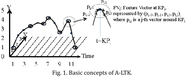
The basic concepts are illustrated in Fig. 1. First, only those time points which are necessary for representing multi-dimensional time-series are selected and used as time-series approximation. The remaining time points are those around which local features are constructed and named keypoints. No features are constructed at the removed time points what were removed.
Fig. 1. Basic concepts of A-LTK.
The purpose of thinned-out keypoints is to represent an original multi-dimensional time series using vectors that are as small as possible. Extraction of a smaller number of keypoints can reduce the computational cost to calculate a dynamic programming scheme such as that used in DTW or LCS.
The purpose of local feature extraction is to retain time series characteristics from locality viewpoints. It is of course important to retain global characteristics in a time series. Using A-LTK, the global characteristics can be represented by combining the local features.
Fig. 2. An example of A-LTK. Fig. 3. A-LTK (Local feature vectors).
which are the prior direction and the next direction, indicate the original time series characteristics. Therefore, these characteristics can be represented with a sequence of local feature vectors at keypoints, as shown in Fig. 3.
3.2.
Thinned-out Keypoints
The features of the technique of out processing are briefly described here. Two types of thinned-out conditions are introduced to select keypoints, namely, a condition on difference with the average and a condition on the second difference.
First, determining whether the condition on the difference with the average is met, given a time point ti, is composed of the following three steps: 1) the average vector avg(ti) is calculated, 2) the difference between vi and avg(ti) is checked, 3) if |vi-avg(ti)| is greater than a predefined threshold 1, then this time
point ti is regarded as a keypoint.
Second, determining whether the condition on the second difference is met, given a time point ti, is composed of the following two steps: 1) the second difference 2(ti) is calculated, where 2(ti) is the
difference of the first difference 2(ti)= (ti+1)-(ti) and (ti)=vi-vi-1, 2) if |2(ti)| is less than a predefined
threshold 2, then the time point ti is treated as a keypoint.
Fig. 4. A condition on the difference with the average. Fig. 5. A condition on the second difference.
Fig. 4 and 5 show examples of the two conditions.
As the setting that is selected for these two thresholds affects the number of keypoints, the thresholds should be determined by using the ratio of the number of keypoints to the total number of time points, that is (#_of_keypoints) / (#_of_time_points). This ratio parameter is defined as the -ratio and has a value in the range of 0.0 to 1.0. Given the -ratio, the respective values of 1 and 2 are set so as to extract
(#_of_keypoints * -ratio /2).
Although the above method for extracting thinned-out keypoints is introduced here for the first time, there are other method that serve the same purpose that could also be applied in our method, such as piecewise linear approximation and approximation by spline functions. They will be employed in future research.
3.3.
Local Feature Constructions
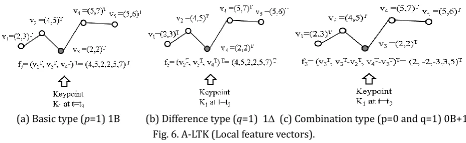
Once a set of keypoints is selected, a feature vector is constructed for each keypoint. As many types of feature vectors can be defined, the description presented here is limited to those that are 1) basic, 2) difference, 3) combination of 1) and 2).
value vectors can be added to the value vector vk. In general, the p-degree (basic) feature vector is defined as (vk-p-1 T, .., vk-1 T, vk T, vk+1 T, ..., vk+p-1 T)T with (2p+1)*d as its vector degree. This type of feature vector is
named pB.
The simple difference type of feature vectors is defined as follows: fk, which is a feature vector at a keypoint Kj (=tk) is fk = (vk T-vk-1 T, vk+1 T-vk T)T. Therefore, in general, q-degree (difference) feature vector is defined by (vk-q-1 T-vk-q T, vk T-vk-1 T, vk+1 T-vk T, vk+qT-vk+q-1 T)T with 2q*d as its vector degree. This type of
feature vector is named q.
The combination type of feature vectors is a combination of p-degree basic vector and q-degree difference vector, with a vector degree of 2p+2q-1. This type of feature vectors is named pB+q.
(a) Basic type (p=1) 1B (b) Difference type (q=1) 1 (c) Combination type (p=0 and q=1) 0B+1
Fig. 6. A-LTK (Local feature vectors).
Fig. 6 shows some examples of these two conditions for the specific cases of 1B, 1, and 0B+1. These three types of local features were introduced, because 1) the conventional time series are represented by a vector whose i-th element are a value at the i-th time, therefore the value can also be used as a local feature; and 2) as in some types of time series such as stock price trends or moving object trajectories, it is necessary to capture value change information, therefore its difference element should be taken into consideration as the local features. However, it should be noted that the higher the values of p or q, the larger the storage cost for local features.
Then, using the local features that were constructed, an approximated sequence, AS(TS), of the original multi-dimensional time series, TS, is defined as follows: the j-th element of the sequence of AS(TS), aj, is a vector fkat a time tksuch that tk is the j-th keypoint. For example, suppose that two keypoints t=t2 and t=t4
are extracted for a TS=<v1, v2, v3, v4, v5>. The approximated sequence of this TS, AS(TS) is <a1, a2>, where a1
and a2 are local feature vectors at t=t2 and t=t4, respectively.
3.4.
Multi-dimensional Time Series Approximation and Applications
First, a similarity function is introduced using our A-LTK. A similarity function SimA-LTK (AS1, AS2), where
AS1=<a1, ..., aN> and AS2=<b1, ..., bM> is defined as follows:
0 0
, ) ,
( 1 2
AS AS if N and M
SIMA LTK
0
0
,
0
)
,
(
1 2
AS
AS
if
N
or
M
SIM
ALTKThe above definition is similar to the definition of DTW, which was described previously.
Secondly, A-LTK can be used to classify a multi-dimensional time series using the above similarity function. The simple classification task is 1-NN, where, given a time series TS, after finding the most similar time series from the database, the class of the found data is considered to be a class of the given data. When the A-LTK is applied to perform clustering of multi-dimensional time series, the above similarity definition can also be used to calculate the distance between two series. In this case any clustering method can be employed, such as K-Means, DB-Scan or a hierarchical clustering method.
Lastly, subsequent searching can be realized based on our A-LTK in the same way as for other methods. Suppose two long multi-dimensional time series are given and A-LTK is used to calculate the similarity between the two. After similar pairs of keypoints are detected, the longest interval of contiguous detected similar pairs can be determined. The details are beyond the scope of this paper. The 1-NN classification task, which is a basic and simple application of time series for comparison, will be considered in the next evaluation section.
4.
Evaluations
4.1.
Test Data Set
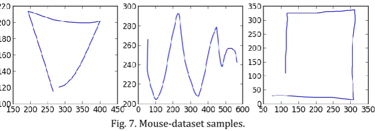
Two dataset: the Dataset and the Mixed-2D-Dataset, were used in our experiments. The Mouse-Dataset contains the sketches of simple pictures, and is composed of four categories: circles, squares, triangles, and waves. Some examples of this dataset are shown in Fig. 7. The number of data items in each category is 20. The Mixed-2D-Dataset was constricted by collecting trajectory data from eight different application fields where each field contains four trajectories of different lengths. Some data in this dataset were extracted from UCR Time series [13]. As these experiments were conducted as preliminary experiments, we only focused on two-dimensional time series. The experiments of multi-dimensional time series with more than three dimensions are underway.
Fig. 7. Mouse-dataset samples.
4.2.
Expriments
The following four experiments were conducted: thinned-out accuracy (EX1), 1-NN processing time (EX2T), 1-NN accuracy (EX2A), and clustering accuracy (EX3). The Mouse Dataset was used for EX1, EX2T, and EX2A, while the Mixed-2D Dataset was used for EX3.
EX1: This experiment checks the extent to which the expected keypoints were able to approximate the original multi-dimensional data, depending on -ratio values. The approximation error for each time series is defined as the following:
1
/
n
(
id
(
v
i,
interpolat
ion
i)
/
v
i)
,interpolationi is the interpolated value at a time point i which is calculated from two vectors at the two
closest keypoints. The average of the error was calculated at the end.
EX2T: This experiment determined the processing time required for 1-NN test using the Mouse-Dataset. The performance of our A-LTK was compared with those of the DTW and AMSS methods. In addition, five variations of A-LTK were compared by changing the -ratio values.
EX2A: This experiment checks the 1-NN classification test from the standpoint of its accuracy using the Mouse-Dataset. The accuracy is defined as (Number of successful classification) / (Number of classification trials). The number of trials equaled to the number of test data set was is 80. The accuracy of the five A-LTK variations was also compared with that of the DTW and AMSS methods.
EX3: This experiment checked the clustering accuracy of the A-LTK compared with DTW and AMSS using the Mixed-2D-Dataset. The accuracy in this experiment was defined as the average of the accuracy for each obtained cluster Ricompared with the actual cluster Ah including the maximal common data as follows:
i
(
max
hR
iA
h/
R
i)
The Ward method is used to do clustering in EX3.
4.3.
Environment
Our experiment was performed in a Windows 7 (Pro) PC with the following specifications: Intel Core i5 3.0GHZ, 8GB Memory, 0.5TB Hard-disk.
4.4.
Results
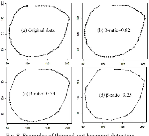
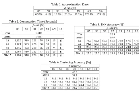
EX1: The results of EX1 are shown in Fig. 8 and Table 1. As shown in the Fig. 8, the shape almost retained its original shape even when a lot of data was removed. A smaller number of keypoints were enough to represent the original data. Table 1 contains the result of approximation accuracy determination with -ratio values. From this table, it is obvious that it is possible to maintain the accuracy even when a small -ratio (=0.036) is used.
Fig. 8. Examples of thinned-out keypoint detection.
processing time are ascribed to a dynamic programming computational cost, O(n2) in general. A shorter
processing time is considered preferable provided the accuracy is maintained. EX2A was designed to verify this.
Table 1. Approximation Error
-ratio(%)
85 58 38 22 13 6.9 3.6
0.35% 6.1% 16.5% 23.3% 32.3% 123.1% 153.1%
Table 2. Computation Time (Seconds)
-ratio(%)
85 58 38 22 13 6.9 3.6
DTW 1,410
AMSS 1,445
1Δ 1,132 519 223 78 29 10 6
2Δ 1,123 523 226 80 30 10 6
1B 1,015 492 218 75 30 9 6
5B 1,065 519 222 77 31 10 6
5B+1Δ 1,184 518 226 78 30 10 6
Table 3. 1NN Accuracy (%)
-ratio(%)
85 58 38 22 13 6.9 3.6
DTW 22.5
AMSS 50.0
1Δ 75.0 62.5 50.0 50.0 70.0 57.5 47.5 2Δ 76.3 68.8 50.0 70.0 70.0 57.5 45.0 1B 25.0 25.0 25.0 23.8 25.0 23.8 25.0 5B 25.0 25.0 25.0 23.8 25.0 23.8 25.0 5B+1Δ 25.0 25.0 25.0 23.8 25.0 23.8 25.0
Table 4. Clustering Accuracy (%)
-ratio(%)
85 58 38 22 13 6.9 3.6
DTW 43.8
AMSS 34.3
1Δ 34.3 34.3 34.3 34.3 34.3 34.3 34.3 1B 43.8 43.8 43.8 46.9 43.8 43.8 37.5 5B 46.9 43.8 43.8 43.8 53.1 40.6 40.6 5B+1Δ 43.8 43.8 43.8 46.9 43.8 40.6 43.8
EX2T: The processing time is shown in Table 2 from which it is clear that the DTW and AMSS required much more processing time compared with A-LTK when the -ratio values were small. The longer processing time are ascribed to a dynamic programming computational cost, O(n2) in general. A shorter
processing time is considered preferable provided the accuracy is maintained. EX2A was designed to verify this.
EX2A: Table 3 shows the result of the 1-NN classification accuracy determination. These results show that the accuracy of the A-LTK method is similar or superior to that obtained by DTW and AMSS methods even when small -ratio values were used, such as -ratio=0.013 or 0.069 in the case of 1Δ and 2Δ. The highest accuracy was obtained in the case of A-LTK(2Δ) with -ratio=0.85.
EX3: In Table 4, the clustering accuracy results are shown. The results show that the A-LTK (5B) method with a -ratio=0.13 obtained the best results in the clustering accuracy experiment. The second best results were obtained from A-LTK (1B) and A-LTK (5B+1Δ) with a -ratio of 0.22. This means that the accuracy displayed by A-LTK(1Δ) was similar to that of AMSS, although worse than that of DTW.
From these experiments, it can be concluded that 1) thinned-out keypoints lead to an improved approximation and thus a smaller processing cost requirement and 2) local features at keypoints improve the accuracy of classification and clustering.
5.
Conclusion and Future Work
capable of attaining similar or superior accuracy compared with other existing methods with the additional advantage of a smaller processing cost.
Our future work include more detailed experiments using time series with more than three dimensions, as well as a dataset from a real application.
Acknowledgment
This work was partially supported by JSPS Grant Number 24300039 and by MEXT-Supported Program for the Strategic Research Foundation at Private Universities 2013-2017.
References
[2] Ho, S.-S., Tang W., & Liu, W. T. (2010). Tropical cyclone event sequence similarity search via dimensionality reduction metric learning. Proceedings of ACM KDD2010 (pp. 135-144).
[11]Tanaka, Y., Iwamoto, K., & Uehara, K. (2005). Discovery of time-series motif from multi-dimensional data based on MDL principle. Machine Learning, 58(2-3), 269-300,
[12]Chakrabarti, K., Keogh, E., Mehrotra, S. & Pazzani, M. (2002). Locally adaptive dimensionality reduction for indexing large time series databases, ACM Trans. Database Syst., 27(2), 188-228.
[13]Keogh, E., Zhu, Q., Hu, B., Hao, Y., Xi, X., Wei L., & Ratanamahatana, C. A. (2011). From The UCR Time Series Classification/ Clustering, Homepage: http://www.cs.ucr.edu/ ~eamonn/time_series_data/
Yu Fang received the B.S. degree from Dalian Jiaotong University in 2013. Her research interests are in the area of databases and data mining.
[3] Chen, Y., et al. (2002). Multi-dimensional regression analysis of time-series data streams. Proceedings of the 28th International Conference on Very Large Data Bases.
[4] Vlachos, M., Hadjieleftheriou, M., Gunopulos, D., & Keogh, E. (2003). Indexing multi-dimensional time-series with support for multiple distance measures. Proceedings of the Ninth ACM SIGKDD International Conference on Knowledge Discovery and Data Mining (pp. 216-225).
[5] Keogh, E., Chakrabarti, K., Pazzani, M., & Mehrotra, S. (2000). Dimensionality reduction for fast similarity search in large time series databases. Journal of Knowledge and Information Systems,3, 263– 286.
[6] Vahdatpour, A., Amini, N., & Sarrafzadeh, M. (2009). Toward unsupervised activity discovery using multi-dimensional motif detection in time series. Proceedings of IJCAI 2009 (pp. 1261-1266).
[7] Holt, G. T., Reinders, M., & Hendriks, E. (2007). Multi-dimensional dynamic time warping for gesture recognition, Proceedings of Annual Conference on the Advanced School for Computing and Imaging. [8] Vlachos, M., Kollios, G., & Gunopulos, D. (2002). Discovering similar multidimensional trajectories.
Proceedings of International Conference on Data Engineering (pp. 673-684).
[9] Chen, L., & Ng, R. (2004). On the marriage of Lp-norms and edit distance. Proceedings of the Thirtieth International Conference on Very Large Data Bases (pp. 792-803).
[10]Nakamura, T., Taki, K., Nomiya, H., & Uehara, K. (2008). AMSS: A similarity measure for time series data.
IEICE Transactions on Information and Systems, J91-D(11), 2579-2588.
Hung-Hsuan Huang received his B.Sc. degree in computer science from National Chen-Chi University, Taiwan in 1998 and the M.Sc. degree from National Taiwan University, Taiwan in 2000. He received his PhD degree from the Kyoto University in 2009. Currently he is an associate professor at the Ritsumeikan University, Japan. His research interests include embodied conversational agent and multimodal HCI. He is one of the members of JSAI, IPSJ, HIS, ACM, and IEICE.