ISSN (e): 2250-3021, ISSN (p): 2278-8719
Vol. 06, Issue 06 (June. 2016), ||V1|| PP 08-20
Use of Polynomial Shape Function in Shear Deformation Theory
for Thick Plate Analysis
1
Ibearugbulem, Owus M.,
2Gwarah,
Ledum S.,
3Ibearugbulem, C. N.
1,2,3 Civil Engineering Department, Federal University of Technology, Owerri, Nigeria
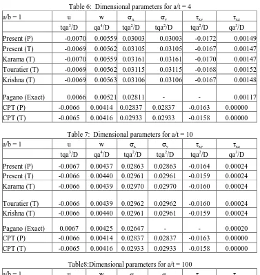
ABSTRACT:-This paper presents use of polynomial shape function in shear deformation theory for thick plate analysis. Total potential energy equation of a thick plate was formulated from the first principle. This equation was subjected to direct variation to obtain three simultaneous direct governing equations for determination of displacement coefficients. Shape (profile) equation for vertical shear stress through the thickness of the plate was formulated from the first principle. From this profile equation, the deformation line equation (called function of z or s) was obtained. This is the model from this study. A numerical problem for a rectangular plate simply supported around all the edges was used to test the sufficiency of this study. Both polynomial and trigonometric shape functions were used in this problem. Three other models were also used. The center deflection - w(0.5, 0.5, 0), in-plane normal x directed stress x(0.5, 0.5, 0.5) and x directed vertical shear stress
xz(0, 0.5, 0) from the present study for span-depth ratio of 4 of a square plate using polynomial shape function are 0.0055 qa4/D, 0.03 tqa2/D and 0.00149 qa3/D. D is plate flexural rigidity, t is plate thickness, q is the uniformly distributed normal load on plate and a is the primary span of the plate. When Trigonometric shape function is used, the values are 0.0056 qa4/D, 0.031 tqa2/D and 0.00147 qa3/D. These are comparable with the value from Pagano (Exact): 0.0052 qa4/D, 0.0281 tqa2/D and 0.00117 qa3/D. It is observed that at span-depth ratio of up to 100 the values based on all the models used herein coincide with the Classical plate theory (CPT) values. The values of from CPT based on polynomial shape function are 0.00414 qa4/D, 0.0283 tqa2/D and 0.00 qa3/D.
Keywords:
shear deformation, vertical shear stress, stress, deflection, displacement, potential energy
shape function
I.
INTRODUCTION
Refined plate theories have been characterized by the use of trigonometric displacement function. Many scholars have obtained the closed form solutions and others have obtained approximate solution by use of energy method. However, one thing is common in them all - the use of trigonometric displacement functions to approximate the deformed shapes of the plates. (Chikalthankar et al., 2013; Sayyad, 2011; Akavci, 2007; Sayyad and Ghugal, 2012; Sadrnejad et al., 2009; Daouadji et al.,2013;Hashemi and Arsanjani, 2005; Reddy, 2014; Shimpi and Patel, 2006; Murthy, 1981; Daouadji, Tounsi, Hadji, Henni and El Abbes, 2012; Zhen-qiang, Xiu:xi and Mao-guang, 1994). Others have applied the polynomial displacement functions in numerical methods like finite element method and differential quadrature element methods (Matikainen, Schwab and Mikkola, 2009;Goswami and Becker, 2013, Liu, 2001). In the course of development of refined plate theory, the assumption that the shear deformation line is not varying linear with depth of the plate was introduced. This according to many scholars helps to ensure that the vertical shear stress across the plate section does not remain constant, but varies parabolically with zero values at both the top and bottom surfaces (Kruszewski, 1949; Ambartsumian, 1958 Krishna, 1984; Touratier, 1991; Karama and Mistou, 2003; Sayyad, 2011). They came up with different shear deformation line functions, here-in-after called F(z). However, there F(z) were not strictly based on the vertical shear stress mathematical formulation. If we follow the work of Timoshenko (Timoshenko and Woinowsky-krieger, 1970), we shall note that maximum shear stress occurs at the mid surface (where z = 0) and the value of maximum shear stress is one and half of vertical shear stress. With most of the F(z) from the literature, we may obtain good profile (curve) for the deformation line and shear stress distribution across the section, but the mid surface value of shear stress may not coincide with that from Timoshenko. Thus, the two specific objectives of the present study include
II.
ASSUMPTIONS
i. The displacements, u, v and w are small when compared with plate thickness.
ii. The in-plane displacements, u and v are differentiable in x, y and z axes, while the out-of-plane displacement (deflection), w is only differentiable in x and y axes. This means that the first derivative of w with respect to z is zero. Consequently, z = 0.
iii. The effect of the out-of-plane normal stress on the gross response of the plate is small when compared with other stresses. Thus, it can be neglected. That is z = 0.
iv. The vertical line that is initially normal to the middle surface of the plate before bending is no longer straight nor normal to the middle surface after bending. That is ≠ c. where is the total rotation of the middle surface in this case, c is the classical plate theorem rotation of the middle surface.
III.
KINEMATIC RELATIONS
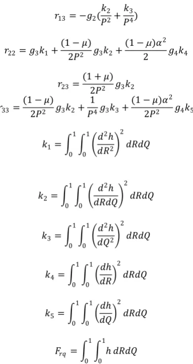
The refined plate theory (RPT) in-plane displacements, u and v as presented on figure 1are defined mathematically as
𝑢 = 𝑢𝑐+ 𝑢𝑠 (1) 𝑣 = 𝑣𝑐+ 𝑣𝑠 (2)
Where u and v are in-plane displacements in x and y directions respectively. The classical in-plane displacements are commonly defined as:
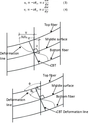
𝑢𝑐= −𝑧𝜃𝑐𝑥 = 𝑧
𝑑𝑤
𝑑𝑥 (3)
𝑣𝑐= −𝑧𝜃𝑐𝑦 = 𝑧𝑑𝑤
𝑑𝑦 (4)
Figure 1: Deformation of a section of a thick plate
z
u
su
cu
Middle surface
Bottom fiber
Top fiber
Deformation
line
CBT
Deformation line
c
sMiddle surface
Bottom fiber
Top fiber
Deformation
line
Analogously, the shear deformation components of the in-plane displacements are defined as:
𝑢𝑠= 𝐹(𝑧)𝜃𝑠𝑥 (5) 𝑣𝑠 = 𝐹(𝑧)𝜃𝑠𝑦 (6)
NoteF(z) is used instead of z. This is because of the fourth assumption (see figure 1). Let us define the deflection (out-of-plane displacement), w as:
𝑤 = 𝑐1ℎ (7)
Substituting equation (7) into equations (3) and (4) gives respectively:
𝑢𝑐= −𝑧 𝑑
𝑑𝑥 𝑐1ℎ = −𝑧𝑐1 𝑑ℎ
𝑑𝑥 (8) 𝑣𝑐= −𝑧
𝑑
𝑑𝑦( 𝑐1ℎ) = −𝑧𝑐1 𝑑ℎ
𝑑𝑦 (9)
Let us mimic expressions in equations (8) and (9) rewrite equations (5) and (6) as:
𝑢𝑠= 𝐹(𝑧)𝑐2 𝑑ℎ
𝑑𝑥 (10)
𝑣𝑠= 𝐹(𝑧)𝑐3𝑑ℎ
𝑑𝑦 (11)
Where c1, c2 and c3 are coefficients of deflection (w), shear deformation rotations (sx and sy). Substituting equations (3) and (10) into equation (1) gives:
𝑢 = −𝑐1𝑧 + 𝑐2𝐹(𝑧) 𝑑ℎ
𝑑𝑥 (12)
Similarly, substituting equations (4) and (11) into equation (2) gives:
𝑣 = −𝑐1𝑧 + 𝑐3𝐹(𝑧) 𝑑ℎ
𝑑𝑦 (13) Strain - Displacement Relations
It was assumed that z is equal to zero. Thus, the remaining five engineering strain components are defined as:
𝑥 = 𝑑𝑢
𝑑𝑥= −𝑐1𝑧 + 𝑐2𝐹(𝑧)
𝑑2ℎ 𝑑𝑥2 (14)
𝑦 = 𝑑𝑣
𝑑𝑦= −𝑐1𝑧 + 𝑐3𝐹(𝑧) 𝑑2ℎ 𝑑𝑦2 (15)
𝑥𝑦 = 𝑑𝑢
𝑑𝑦+
𝑑𝑣
𝑑𝑥= −𝑐1𝑧 + 𝑐2𝐹(𝑧)
𝑑2ℎ
𝑑𝑥𝑑𝑦+ −𝑐1𝑧 + 𝑐3𝐹(𝑧)
𝑑2ℎ 𝑑𝑥𝑑𝑦
= −2𝑐1𝑧 + 𝑐2𝐹 𝑧 + 𝑐3𝐹(𝑧) 𝑑
2ℎ
𝑑𝑥𝑑𝑦 (16)
𝑥𝑧 = 𝑑𝑢
𝑑𝑧+
𝑑𝑤 𝑑𝑥
= −𝑐1+ 𝑐2 𝑑𝐹 𝑧
𝑑𝑧 𝑑ℎ 𝑑𝑥+ 𝑐1
𝑑ℎ 𝑑𝑥
That is
𝑥𝑧 = 𝑐2𝑑𝐹 𝑧 𝑑𝑧
𝑑ℎ
𝑑𝑥 (17)
𝑦𝑧 = 𝑑𝑣
𝑑𝑧+
𝑑𝑤 𝑑𝑦
= −𝑐1+ 𝑐3𝑑𝐹 𝑧
𝑑𝑧 𝑑ℎ
𝑑𝑦+ 𝑐1
𝑑ℎ 𝑑𝑦
That is
𝑦𝑧 = 𝑐3𝑑𝐹 𝑧 𝑑𝑧
𝑑ℎ
𝑑𝑦 (18)
IV.
CONSTITUTIVE RELATIONS
𝑥 = 𝐸
1 −2 𝑥+ 𝑦 (19)
𝑦 = 𝐸
1 −2 𝑥+ 𝑦 (20)
𝑥𝑦 =
𝐸(1 −)
1 −2 𝑥𝑦 (21) 𝑥𝑧 =
𝐸(1 −)
1 −2 𝑥𝑧 (22)
𝑦𝑧 =
𝐸(1 −)
1 −2 𝑦𝑧 (23)
V.
STRESS – DISPLACEMENT EQUATIONS
Substituting equations (14) to (18) into equations (19) to (23) where appropriate gives:
𝑥 = 𝐸
1 −2 −𝑐1𝑧 + 𝑐2𝐹(𝑧)
𝑑2ℎ
𝑑𝑥2+ −𝑐1𝑧 + 𝑐3𝐹(𝑧) 𝑑2ℎ
𝑑𝑦2 (24)
𝑦 = 𝐸
1 −2 𝑧 𝑐1+ 𝐹(𝑧)
𝑧 𝐵2
𝑑2ℎ
𝑑𝑥2+ −𝑐1𝑧 + 𝑐3𝐹(𝑧)
𝑑2ℎ
𝑑𝑦2 (25)
𝑥𝑦 =
𝐸(1 −)
2 1 −2 −2𝑐1𝑧 + 𝑐2𝐹 𝑧 + 𝑐3𝐹(𝑧)
𝑑2ℎ
𝑑𝑥𝑑𝑦 (26)
𝑥𝑧 =
𝐸(1 −)
2 1 −2 𝑐2 𝑑𝐹 𝑧
𝑑𝑧 𝑑ℎ
𝑑𝑥 (27)
𝑦𝑧 =
𝐸(1 −)
2 1 −2 𝑐3
𝑑𝐹 𝑧 𝑑𝑧
𝑑ℎ
𝑑𝑦 (28)
VI.
TOTAL POTENTIAL ENERGY
Total potential energy is the summation of strain energy, U and external work, V. that’s
= 𝑈 + 𝑉 (29)
Let’s define external work as:
𝑉 = −𝑞 𝑤 𝑦 𝑥
𝑑𝑥𝑑𝑦 (30)
Let’s also define strain energy mathematically:
𝑈 = .𝑑𝑧
𝑡 2
−𝑡 2 𝑦 𝑥
𝑑𝑥𝑑𝑦
= 𝑥𝑥+𝑦𝑦+𝑥𝑦𝑥𝑦 +𝑥𝑧𝑥𝑧+𝑦𝑧𝑦𝑧 𝑑𝑧 𝑡
2
−2𝑡 𝑦 𝑥
𝑑𝑥𝑑𝑦 (31)
Using equations (14) and (24), (15) and (25), (16) and (26), (17) and (27), and (18) and (28) respectively gives:
𝑥𝑥 = 𝐸 1 −2 𝑧
2𝑐12− 2𝑐1𝑐2𝑧𝐹(𝑧) + 𝑐22𝐹(𝑧)2 𝑑 2ℎ
𝑑𝑥2 2
+ 𝑧2𝑐
12− 𝑐1𝑐2𝑧𝐹 𝑧 − 𝑐1𝑐3𝑧𝐹(𝑧) + 𝑐2𝑐3𝐹(𝑧)2 𝑑2ℎ 𝑑𝑥𝑑𝑦
𝑦𝑦 = 𝐸 1 −2 𝑧
2𝑐12− 2𝑐1𝑐3𝑧𝐹(𝑧) + 𝑐32𝐹(𝑧)2 𝑑 2ℎ
𝑑𝑦2 2
+ 𝑧2𝑐12− 𝑐1𝑐2𝑧𝐹 𝑧 − 𝑐1𝑐3𝑧𝐹(𝑧) + 𝑐2𝑐3𝐹(𝑧)2 𝑑 2ℎ
𝑑𝑥𝑑𝑦 2
(33)
𝑥𝑦.𝑥𝑦 =
𝐸(1 −)
2 1 −2 4𝑐1
2𝑧2− 4𝑐1𝑐2𝑧𝐹 𝑧 − 4𝑐1𝑐3𝑧𝐹 𝑧 + 𝑐22𝐹(𝑧)2+ 2𝑐2𝑐3𝐹(𝑧)2
+ 𝑐32𝐹(𝑧)2 𝑑 2ℎ
𝑑𝑥𝑑𝑦 2
(34)
𝑥𝑧.𝑥𝑧 =
𝐸(1 −)
2 1 −2 𝑐22 𝑑𝐹(𝑧)
𝑑𝑧 2
𝑑ℎ 𝑑𝑥
2
(35)
𝑦𝑧.𝑦𝑧 =
𝐸(1 −)
1 −2 𝑐32 𝑑𝐹(𝑧)
𝑑𝑧 2
𝑑ℎ 𝑑𝑦
2
(36)
Substituting equations (32) to (36) into equation (31) gives:
𝑈 = 𝐷
2 [𝑥 𝑦 𝑔1𝑐1 2− 2𝑔
2𝑐1𝑐2+ 𝑔3𝑐22] 𝑑2ℎ 𝑑𝑥2
2
+ 2𝑔1𝑐12− 2𝑔2𝑐1𝑐2− 2𝑔2𝑐1𝑐3+1
2𝑔3𝑐2
2+ 𝑔3𝑐2𝑐3+1
2𝑔3𝑐3 2 𝑑
2ℎ
𝑑𝑥𝑑𝑦 2
+ 𝑔3𝑐2𝑐3−1 2𝑔3𝑐2
2−1 2𝑔3𝑐3
2 𝑑 2ℎ
𝑑𝑥𝑑𝑦 2
+ 𝑔1𝑐12− 2𝑔2𝑐1𝑐3+ 𝑔3𝑐32 𝑑2ℎ 𝑑𝑦2
2
+(1 −)𝛼
2
2 𝑔4𝑐2
2 𝑑ℎ 𝑑𝑥
2
+ 1 − 𝛼
2
2 𝑔4𝐵3
2 𝑑ℎ 𝑑𝑦
2
] 𝑑𝑥𝑑𝑦 (37)
Where:
𝐷 = 𝑡 3
12
𝑔1=
𝑧2𝑑𝑧
𝑡 2 −2𝑡
𝐷 = 1 (38)
𝑔2=
𝑧𝐹 𝑧 𝑑𝑧 𝑡
2 −𝑡
2
𝐷 (39)
𝑔3=
𝐹(𝑧)2𝑑𝑧
𝑡 2 −𝑡2
𝛼2𝑔 4=
𝑑𝐹 (𝑧)𝑑𝑧 2𝑑𝑧 𝑡
2 −2𝑡
𝐷 (41)
The flexural rigidity of the plate is:
𝐷 = 𝐸
1 −2∗ 𝐷 = 𝐸𝑡3
12(1 −2)(42)
Let’s define the span-depth aspect ratio as
=𝑎
𝑡 (43)
Where a and t are the primary span (length in x direction, while b is the length in y direction) of the plate and plate thickness respectively.
Let define non dimensional coordinates R and Q and the span-span aspect ratio, P as:
𝑅 =𝑥
𝑎𝑥 = 𝑎𝑅 (44)
𝑄 =𝑦
𝑏𝑦 = 𝑏𝑄 (45)
𝑃 =𝑏
𝑎𝑏 = 𝑎𝑃 (46)
Substituting equations (30), (37) and (43) to (46)into equation (29) gives:
=𝑎𝑏𝐷
2𝑎4 [
1
0 1
0
𝑔1𝑐12− 2𝑔2𝑐1𝑐2+ 𝑔3𝑐22] 𝑑2ℎ 𝑑𝑅2
2
+ 1
𝑃2 2𝑔1𝑐12− 2𝑔2𝑐1𝑐2− 2𝑔2𝑐1𝑐3 𝑑2ℎ 𝑑𝑅𝑑𝑄
2
(1 + 𝜇) 𝑃2 𝑔3𝑐2𝑐3
𝑑2ℎ 𝑑𝑅𝑑𝑄
2
+(1 −)
2𝑃2 𝑔3𝑐22+ 𝑔3𝑐32 𝑑2ℎ 𝑑𝑅𝑑𝑄
2
+(1 −)𝛼
2
2 𝑔4𝑐2
2 𝑑ℎ 𝑑𝑅
2
+(1 −)𝛼
2
2𝑃2 𝑔4𝑐3
2 𝑑ℎ 𝑑𝑄
2 ] 𝑑𝑅𝑑𝑄
−𝑎𝑏 𝐹𝐹 1
0 1
0
𝑑𝑅𝑑𝑄 (47)
VII.
DIRECT GOVERNING EQUATIONS
This total potential energy contains three unknown coefficients (c1, c2 and c3) for deflection, rotation in x axis and rotation in y axis. Differentiating total potential energy equation with respect to c1, c2 and c3 in turn will give three simultaneous equations.
𝑑
𝑑𝑐1 =
𝑑
𝑑𝑐2=
𝑑
𝑑𝑐3= 0 (48)
Substituting equation (47) into equation (48) gives in matrix form:
𝑟11 𝑟12 𝑟13 𝑟12 𝑟22 𝑟23 𝑟13 𝑟23 𝑟33
𝑐1 𝑐2 𝑐3
=𝑎
4
𝐷 𝐹𝑟𝑞
0 0
(49)
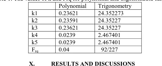
Where
𝑟11= 𝑔1(𝑘1+ 2
𝑘2 𝑃2+
𝑘3 𝑃4)
𝑟13= −𝑔2( 𝑘2 𝑃2+
𝑘3 𝑃4)
𝑟22= 𝑔3𝑘1+ (1 − 𝜇)
2𝑃2 𝑔3𝑘2+
(1 −)𝛼2
2 𝑔4𝑘4
𝑟23=
(1 + 𝜇) 2𝑃2 𝑔3𝑘2
𝑟33=
(1 − 𝜇) 2𝑃2 𝑔3𝑘2+
1
𝑃4𝑔3𝑘3+
(1 − 𝜇)𝛼2
2𝑃2 𝑔4𝑘5
𝑘1=
𝑑2ℎ 𝑑𝑅2
2 1
0 1
0
𝑑𝑅𝑑𝑄
𝑘2= 𝑑
2ℎ
𝑑𝑅𝑑𝑄 2 1
0 1
0
𝑑𝑅𝑑𝑄
𝑘3= 𝑑
2ℎ
𝑑𝑄2 2 1
0 1
0
𝑑𝑅𝑑𝑄
𝑘4=
𝑑ℎ 𝑑𝑅
2 1
0 1
0
𝑑𝑅𝑑𝑄
𝑘5=
𝑑ℎ 𝑑𝑄
2 1
0 1
0
𝑑𝑅𝑑𝑄
𝐹𝑟𝑞 = ℎ
1
0 1
0
𝑑𝑅𝑑𝑄
SHEARING STRESS DISTRIBUTION IN RECTANGULAR CROSS-SECTIONS
Figure 2: A rectangular cross section
From strength of materials, the equation shear stress is given as:
𝜏 =𝑉𝐻
𝐼𝑏 (50)
Where V, H, I and b are transverse shear force, first moment of area, second moment of inertia and breadth of the section respectively.
Using figure 2 and following mathematically principle the first moment of area is obtained:
𝐻 = 𝑧 𝑑𝐴 =𝑏
2 𝑡 2− 𝑧
𝑡
2+ 𝑧
N.A
𝑡
2
− 𝑧
b
z
dA
𝑡
That is,𝐻 =𝑏 2
𝑡2 4 − 𝑧
2 (51)
The second moment of inertia for a rectangular section is given as:
𝐼 =𝑏𝑡
2
12 (52)
Substituting equations (51) and (52) into equation (50) gives:
𝜏 = 𝑉
𝑏𝑡 3
2− 6
𝑧 𝑡2
2
= 𝑉
𝑏𝑡𝐺(𝑧) (53)
Where the shear stress profile, G(z) is:
𝐺 𝑧 = 3
2− 6
𝑧 𝑡2
2
(54)
It is assumed here that the shear stress profile, G(z) is related to shear deformation profile, F(z) as:
𝐺 𝑧 = 𝑑𝐹(𝑧)
𝑑𝑧 (55)
Using equations (54) and (55) we obtain:
𝐹 𝑧 =3𝑧
2 1 −
4 3
𝑧 𝑡 2
(56)
𝐹 𝑆 =3𝑆𝑡
2 1 −
4 3𝑆
2 (56𝑏)
Where S = z/t (a non-dimensional form of z)
This function of z is exactly Krishna Murty Model (KrishnaMurty, 1984) divided by 1.5. However, using the Krishna Murty model will result in unestimating the vertical shear stress by 50%.
Substituting F(S) models into equations (39) to (41) gives g1, g2, g3 and g4 values for different models used herein for numerical examples:
i. Present Model
𝐹 𝑆 =3𝑆𝑡
2 1 −
4 3𝑆
2
𝑔1= 1; 𝑔2= 1.2; 𝑔3=51
35; 𝑔4= 14.4
ii. Touratier 1991 model
𝐹 𝑆 =𝑡
𝜋sin(𝜋𝑆) 𝑔1= 1; 𝑔2= 0.774; 𝑔3=
307
505; 𝑔4= 6
iii. Karama et al. 2003 model
𝐹 𝑆 = 𝑆𝑡. exp(−2𝑆2)
𝑔1= 1; 𝑔2=344
439; 𝑔3=
274
422; 𝑔4= 6.18744
VIII. DEFINITION OF SOME QUANTITIES Recall equation 7:
𝑤 = 𝑐1ℎ (7)
Let us rewrite it as:
𝑤 = 𝑐1ℎ = 𝐵1ℎ 𝑞𝑎4
𝐷 = 𝑘𝑤 𝑞𝑎4
𝐷
𝑘𝑤= 𝐵1ℎ𝑎𝑛𝑑𝐵1= 𝑞𝑎𝑐14
𝐷
Let the displacements of plate under pure bending then be defined as:
𝑤 = 𝑞𝑎
4
𝐷 𝑘𝑤 (56)
𝑢 = 𝑡𝑞𝑎
3
𝐷 𝑘𝑢 (57)
𝑣 = 𝑡𝑞𝑎
3
𝐷 𝑘𝑣 (58)
Where kw, a and D are as defined earlier, q is the uniform distributed load on the plate. ku and kv are extracted from equations (12) and (13) as:
𝑘𝑢 = −𝐵1𝑆 + 𝐵2𝐹(𝑆) 𝑑ℎ
𝑑𝑅 (59)
𝑘𝑣 =1
𝑃 −𝐵1𝑆 + 𝐵3𝐹(𝑆) 𝑑ℎ
𝑑𝑄 (60)
𝑊ℎ𝑒𝑟𝑒𝐵2=
𝑐2 𝑞𝑎4 𝐷
𝑎𝑛𝑑𝐵3 =
𝑐3 𝑞𝑎4
𝐷
Similarly, let us define the stress components as:
𝜎𝑥= 𝐸
1 − 𝜇2 𝑡𝑞𝑎2
𝐷 𝑘𝜎𝑥 (61)
𝜎𝑦 = 𝐸 1 − 𝜇2
𝑡𝑞𝑎2
𝐷 𝑘𝜎𝑦 (62)
𝜏𝑥𝑦 = 𝐸
1 + 𝜇 𝑡𝑞𝑎2
𝐷 𝑘𝜏𝑥𝑦 (63)
𝜏𝑥𝑧 = 𝐸 1 + 𝜇
𝑞𝑎3
𝐷 𝑘𝜏𝑥𝑧 (64)
𝜏𝑦𝑧 = 𝐸
1 + 𝜇 𝑞𝑎3
𝐷 𝑘𝜏𝑦𝑧 (65)
Where kx, ky, kτxy, kτxz and kτyz are defined from equations (24) to (28)as:
𝑘𝜎𝑥 = −𝐵1𝑆 + 𝐵2𝐹 𝑆 𝑑
2ℎ
𝑑𝑅2+
𝑃2 −𝐵1𝑆 + 𝐵3𝐹(𝑆) 𝑑2ℎ
𝑑𝑄2 (66)
𝑘𝜎𝑌 = −𝐵1𝑆 + 𝐵2𝐹 𝑆 𝑑2ℎ
𝑑𝑅2+
1
𝑃2 −𝐵1𝑆 + 𝐵3𝐹(𝑆)
𝑑2ℎ
𝑑𝑄2 (67)
𝑘𝜏𝑥𝑦 = 1
2𝑃 −2𝐵1𝑆 + 𝐵2𝐹 𝑆 + 𝐵3𝐹(𝑆) 𝑑2ℎ
𝑑𝑅𝑑𝑄 (68)
𝑘𝜏𝑥𝑧 = 𝐵2
2 𝑑𝐹 𝑆
𝑑𝑆 𝑑ℎ
𝑑𝑅 (69)
𝑘𝜏𝑦𝑧 =𝐵3 2𝑃
𝑑𝐹 𝑆 𝑑𝑆
𝑑ℎ
𝑑𝑄 (70)
Substituting equations (42) and (43) into equations (56) to (58) gives:
𝑤 = 12(1 − 𝜇2)3𝑘𝑤 𝑞𝑎
𝐸 (71) 𝑢 = 12(1 − 𝜇2)3𝑘
𝑢 𝑡𝑞
𝐸 (72) 𝑣 = 12(1 − 𝜇2)3𝑘
𝑣 𝑡𝑞
𝐸 (73)
Similarly, substituting equations (42) and (43) into equations (61) to (65) gives:
𝜎𝑥= 𝑘𝜎𝑥 12
2 𝑞 (74)
𝜎𝑦 = 𝑘𝜎𝑦 122 𝑞 (75) 𝜏𝑥𝑦 = 𝑘𝜏𝑥𝑦 12
𝜏𝑥𝑧 = 𝑘𝜏𝑥𝑧 12
3(1 − 𝜇) 𝑞 (77)
𝜏𝑦𝑧 = 𝑘𝜏𝑦𝑧 12
3(1 − 𝜇) 𝑞 (78)
Let us define non-dimensional form of the displacements and stress components according to Sayyad et al. (2012) as:
𝑤 = 100𝐸𝑤
𝑞𝑡4 79 ; 𝑢 = 𝑢𝐸 𝑞𝑡3 80
𝑣 = 𝑣𝐸
𝑞𝑡3 81 ; 𝜎 𝑥= 𝜎𝑥 𝑞2 82 𝜎 𝑦 =
𝜎𝑦
𝑞2 83 ; 𝜏 𝑥𝑦 = 𝜏𝑥𝑦 𝑞2 84 𝜏 𝑥𝑧 =
𝜏𝑥𝑧
𝑞 85 ; 𝜏 𝑦𝑧 = 𝜏𝑦𝑧 𝑞 86
Using equations (71) to (78), we define the non-dimensional form of the displacements and stress components as:
𝑤 = 1200 1 − 𝜇2 𝑘 𝑤 87 𝑢 = 12 1 − 𝜇2 𝑘
𝑢 88 𝑣 = 12 1 − 𝜇2 𝑘
𝑣 89 𝜎 𝑥= 12𝑘𝜎𝑥 90 𝜎 𝑦 = 12𝑘𝜎𝑦 91 𝜏 𝑥𝑦 = 12 1 − 𝜇 𝑘𝜏𝑥𝑦 92 𝜏 𝑥𝑧= 122 1 − 𝜇 𝑘
𝜏𝑥𝑧 93 𝜏 𝑦𝑧 = 122 1 − 𝜇 𝑘𝜏𝑦𝑧 94
IX. NUMERICAL PROBLEM
Determine the deflection at the center (0.5, 0.5, 0) of ssss thick plate. Where (0.5, 0.5, 0) means R = 0.5; Q = 0.5; S = 0. Determine also the in-plane normal stresses at (0.5, 0.5, 0.5), in-plane shear stress at (0, 0, 0.5) and the vertical shear stress (xz) at (0, 0.5, 0) of thessss plate. Polynomial and trigonometric displacement shall be used. Function.
The polynomial displacement function, h is given as:
ℎ = 𝑅 − 2𝑅3+ 𝑅4 𝑄 − 2𝑄3+ 𝑄4 (57)
The trigonometric displacement function, h is given as:
ℎ = sin 𝜋𝑅 sin 𝜋𝑄 (58)
The k values for both polynomial and trigonometric functions are given on table 1.
Table 1: The values of k and Frq for polynomial and trigonometric functions Polynomial Trigonometry
k1 0.23621 24.352273 k2 0.23591 24.35227 k3 0.23621 24.35227 k4 0.0239 2.467401 k5 0.0239 2.467401 Frq 0.04 92/227 X. RESULTS AND DISCUSSIONS
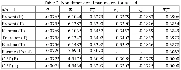
Table 2: Non dimensional parameters for a/t = 4
a/b = 1 𝑢 𝑤 𝜎𝑥 𝜎𝑦 𝜏𝑥𝑦 𝜏𝑥𝑧
Present (P) -0.0765 6.1044 0.3279 0.3279 -0.1883 0.3906 Present (T) -0.0755 6.1383 0.3390 0.3390 -0.1826 0.3854 Karama (T) -0.0769 6.1035 0.3452 0.3452 -0.1859 0.3849 Touratier (T) -0.0758 6.1342 0.3402 0.3402 -0.1832 0.3973 Krishna (T) -0.0756 6.1483 0.3392 0.3392 -0.1826 0.3878 Pagano (Exact) 0.0720 5.6940 0.3070 - - 0.3067 CPT (P) -0.0723 4.5175 0.3098 0.3098 -0.1779 0.0000 CPT (T) -0.0071 4.5434 0.3203 0.3203 -0.1725 0.0000
Legend: (P) means the shape function is polynomial (T) means the shape function is trigonometry Table 3: Non dimensional parameters for a/t = 10
a/b = 1 𝑢 𝑤 𝜎𝑥 𝜎 𝑦 𝜏 𝑥𝑦 𝜏𝑥𝑧
Present (P) -0.0730 4.7723 0.3127 0.3127 -0.1796 0.3920 Present (T) -0.0720 4.7995 0.3233 0.3233 -0.1741 0.3868 Karama (T) -0.0723 4.7970 0.3243 0.3243 -0.1746 0.3909 Touratier (T) -0.0721 4.7991 0.3235 0.3235 -0.1742 0.3991 Krishna (T) -0.0720 4.8011 0.3233 0.3233 -0.1741 0.3892 Pagano (Exact) 0.0730 4.6390 0.2890 - - 0.3247 CPT (P) -0.0723 4.5175 0.30977 0.30977 -0.17792 0.0000 CPT (T) -0.0714 4.5434 0.3203 0.3203 -0.1725 0.0000
Table 4: Non dimensional parameters for a/t = 100
a/b = 1 𝑢 𝑤 𝜎𝑥 𝜎𝑦 𝜏𝑥𝑦 𝜏𝑥𝑧
Present (P) -0.0723 4.5201 0.3098 0.3098 -0.1779 0.3920 Present (T) -0.0714 4.5460 0.3203 0.3203 -0.1725 0.3868 Karama (T) -0.0714 4.5460 0.3203 0.3203 -0.1725 0.3909 Touratier (T) -0.0714 4.5460 0.3203 0.3203 -0.1725 0.3991 Krishna (T) -0.0714 4.5460 0.3203 0.3203 -0.1725 0.3892 CPT (P) -0.0723 4.5175 0.3098 0.3098 -0.1779 0.3247 CPT (T) -0.0714 4.5434 0.3203 0.3203 -0.1725 0.0000
Table 5: Non dimensional parameters for a/t = 1000
a/b = 1 𝑢 𝑤 𝜎 𝑥 𝜎𝑦 𝜏𝑥𝑦 𝜏 𝑥𝑧
Table 6: Dimensional parameters for a/t = 4
a/b = 1 u w x y τxy τxz
tqa3/D qa4/D tqa2/D tqa2/D tqa2/D qa3/D Present (P) -0.0070 0.00559 0.03003 0.03003 -0.0172 0.00149 Present (T) -0.0069 0.00562 0.03105 0.03105 -0.0167 0.00147 Karama (T) -0.0070 0.00559 0.03161 0.03161 -0.0170 0.00147 Touratier (T) -0.0069 0.00562 0.03115 0.03115 -0.0168 0.00152 Krishna (T) -0.0069 0.00563 0.03106 0.03106 -0.0167 0.00148 Pagano (Exact) 0.0066 0.00521 0.02811 - - 0.00117 CPT (P) -0.0066 0.00414 0.02837 0.02837 -0.0163 0.00000 CPT (T) -0.0065 0.00416 0.02933 0.02933 -0.0158 0.00000
Table 7: Dimensional parameters for a/t = 10
a/b = 1 u w x y τxy τxz
tqa3/D qa4/D tqa2/D tqa2/D tqa2/D qa3/D Present (P) -0.0067 0.00437 0.02863 0.02863 -0.0164 0.00024 Present (T) -0.0066 0.00440 0.02961 0.02961 -0.0159 0.00024 Karama (T) -0.0066 0.00439 0.02970 0.02970 -0.0160 0.00024 Touratier (T) -0.0066 0.00439 0.02962 0.02962 -0.0160 0.00024 Krishna (T) -0.0066 0.00440 0.02961 0.02961 -0.0159 0.00024 Pagano (Exact) 0.0067 0.00425 0.02647 - - 0.00020 CPT (P) -0.0066 0.00414 0.02837 0.02837 -0.0163 0.00000 CPT (T) -0.0065 0.00416 0.02933 0.02933 -0.0158 0.00000
Table8:Dimensional parameters for a/t = 100
a/b = 1 u w x y τxy τxz
tqa3/D qa4/D tqa2/D tqa2/D tqa2/D qa3/D Present (P) -0.0066 0.00414 0.02837 0.02837 -0.0163 0.00000 Present (T) -0.0065 0.00416 0.02933 0.02933 -0.0158 0.00000 Karama (T) -0.0065 0.00416 0.02934 0.02934 -0.0158 0.00000 Touratier (T) -0.0065 0.00416 0.02933 0.02933 -0.0158 0.00000 Krishna (T) -0.0065 0.00416 0.02933 0.02933 -0.0158 0.00000 CPT (P) -0.0066 0.00414 0.02837 0.02837 -0.0163 0.00000 CPT (T) -0.0065 0.00416 0.02933 0.02933 -0.0158 0.00000
Table9:Dimensional parameters for a/t = 1000
a/b = 1 u w x y τxy τxz
REFERENCES
[1] S.A. Sadrnejad, A. SaediDaryan and M. Ziaei (2009). Vibration Equations of Thick Rectangular Plates Using Mindlin Plate Theory. Journal of Computer Science 5 (11): 838-842, 2009 ISSN 1549-3636 [2] T. H. Daouadji, A. Tounsi and El A. A. Bedia (2013).A New Higher Order Shear Deformation Model for
Static Behavior of Functionally Graded Plates. Advances in Applied Mathematics and Mechanics Adv. Appl. Math. Mech., Vol. 5, No. 3, pp. 351-364
[3] S. Sayyada Y. M. Ghugal (2012). Bending and free vibration analysis of thick isotropic plates by using exponential shear deformation theory. Applied and Computational Mechanics 6, pp. 65–82
[4] M. V.V. Murthy (1981). An Improved Transverse Shear Deformation Theory for Laminated Anisotropic Plates. NASA Technical Paper 1903
[5] A. S. Sayyad (2011). Comparison of various shear deformation theories for the free vibration of thick isotropic beams. INTERNATIONAL JOURNAL OF CIVIL AND STRUCTURAL ENGINEERING Volume 2, No 1,pp. 85-97
[6] S.H. Hashemi, M. Arsanjani (2005). Exat characteristic equations for some of classical boundary conditions of vibrating moderately thick rectangular plate. International Journal of Solids and Structures 42 (2005) 819–853
[7] S.B.Chikalthankar, I.I.Sayyad, V.M.Nandedkar (2013).Analysis of Orthotropic Plate By Refined Plate Theory. International Journal of Engineering and Advanced Technology (IJEAT) ISSN: 2249 – 8958, Volume-2, Issue-6, pp. 310-315
[8] B. Sidda Reddy (2014).Bending Behaviour Of Exponentially Graded Material Plates Using New Higher
Order Shear Deformation Theory with Stretching Effect . International Journal of Engineering Research ISSN:2319-6890)(online),2347-5013(print) Volume No.3 Issue No: Special 1, pp: 124-131
[9] M. K. Matikainen, A. L. Schwab and Aki M. Mikkola (2009). Comparison of two moderately thick plate elements based on the absolute nodal coordinate formulation. MULTIBODY DYNAMICS 2009, ECCOMAS Thematic Conference K. Arczewski, J. Fra˛czek, M. Wojtyra (eds.) Warsaw, Poland, 29 June–2 July 2009.
[10] T. H.Daouadji, A. Tounsi, L. Hadji, A. H. Henni, A. B. El Abbes (2012). A theoretical analysis for static and dynamic behavior of functionally graded plates. Materials Physics and Mechanics 14 (2012) 110-128 [11] C. Zhen-qiang, W.Xiu:xiand H. Mao-guang (1994). Postbuckling behavior of rectangular moderately
thick plates and sandwich plates. Applied Mathematics and Mechanics (English Edition, Vol. 15, No. 7, July 1994).
[12] R.P. Shimpi, H. G. Patel (2006).A two variable refined plate theory for orthotropic plate analysis. International Journal of Solids and Structures 43 (2006) 6783–6799
[13] S. Goswami, W. Becker (2013). A New Rectangular Finite Element Formulation Based on Higher Order Displacement Theory for Thick and Thin Composite and Sandwich Plates. World Journal of Mechanics, 2013, 3, 194-201
[14] M. A. V. Krishna (1984), Toward a consistent beam theory, AIAA Journal, 22, pp 811-816.
[15] S. A. Ambartsumian (1958), On the theory of bending plates, Izvotd Tech Nauk an Sssr, 5, pp 69–77. [16] E. T. Kruszewski (1949), Effect of transverse shear and rotatory inertia on the natural frequency of a
uniform beam, NACA TN, 1909.
[17] M. Karama, K. S. Afaq and S. Mistou (2003), Mechanical behavior of laminated composite beam by new multi-layered laminated composite structures model with transverse shear stress continuity, International Journal of Solids and Structures, 40, pp 1525–46.
[18] M. Touratier (1991), An efficient standard plate theory, International Journal of Engineering Science, 29(8), pp 901–16.
[19] S. P. Timoshenko, And S. Woinowsky-krieger (1970). Theory of plates and shells (2nd Ed.). Singapore: Mc Graw-Hill Book Co. P.379.