ELM Dynamic Simulation for Detached Divertor Plasmas Using
One-Dimensional Fluid Code
∗
)
Yue LI, Satoshi TOGO
1), Tomonori TAKIZUKA
2)and Yuichi OGAWA
Graduate School of Frontier Sciences, The University of Tokyo, Kashiwa 277-8568, Japan
1)Plasma Research Center, University of Tsukuba, Tsukuba 305-8577, Japan
2)Graduate School of Engineering, Osaka University, Suita 565-0871, Japan
(Received 27 December 2017/Accepted 2 April 2018)
We investigate the dynamic response of plasma detachment against the Edge Localized Mode (ELM) using a one-dimensional fluid code. It is found that the heat flux to the target plate after an ELM crash in the detachment starts to increase with a delay, contrary to the sudden increase in the attachment. Larger electron heat flux and smaller ion heat flux to the plate are found in the detachment due to the strong equipartition between electron and ion temperatures, while their heat fluxes are similar in the attachment. In addition, we find the reverse flow in the detachment caused by ELM unbalancing the plasma pressure. Finally, we examine the grassy-ELMs, and find the accumulation of the heat flux pulses in the detached divertor.
c
2018 The Japan Society of Plasma Science and Nuclear Fusion Research
Keywords: ELM, detached plasma, one-dimensional fluid code, dynamic response, reverse flow DOI: 10.1585/pfr.13.3403054
1. Introduction
For designing the divertor of a next-generation fusion reactor, the most promising method to reduce the diver-tor heat load is the plasma detachment. However, the Edge Localized Mode (ELM) in an H-mode tokamak plasma can affect the plasma detachment [1, 2]. Therefore, it is impor-tant to confirm whether the plasma detachment is still an efficient method or not to control the transiently enhanced heat and particle loads due to ELM.
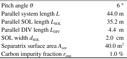
We have been developing a one-dimensional (1D) scrape offlayer - divertor (SOL-DIV) fluid code for study-ing detachment plasma [3]. In this research, we attempt to investigate ELM dynamic behaviors in the plasma de-tachment using a simple 1D code, although the physics of plasma detachment has still not fully been understood and the current divertor simulation codes are applied basically to study static behaviors of plasma detachment. Consider-ing the fact that the characteristics of ELM energy and par-ticle losses have been investigated much in ASDEX Up-grade [4], we use the parameters in Refs. [4–6] for the present research as shown in Table 1.
In this paper, we study ELM dynamic behaviors in the plasma detachment through adjusting amplitudes of ELM to type I ELM and grassy ELMs. In the case of type I ELM, we focus on the effect of fraction of impurity den-sity on the reverse flow which is observed near the target plate. On the other hand, in the case of grassy ELMs, we focus on the radiation effect which makes the difference of ELM heat fluxes between attachment and detachment author’s e-mail: [email protected]
∗)This article is based on the presentation at the 26th International Toki
Conference (ITC26).
Table 1 Basic parameters based on ASDEX Upgrade plasma.
much larger than that in the case of type I ELM.
2. Simulation Model
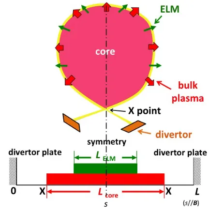
The geometry of this model is shown as Fig. 1. Two divertor plates are located at s =0 and s = L, where s
represents the coordinate in the parallel direction to the magnetic field lines in a tokamak SOL-DIV plasmas.Lcore andLELMdenote the ranges of steady-state core source and pulsed ELM source, respectively. In the present calcula-tion, for simplicity, both sources are given symmetrically in space withLcore=LSOLandLELM=LSOL/2.
We have been developing a 1D plasma fluid model based on the Braginskii equations [7] as shown in Eqs. (1 - 4) for densityn, parallel flow velocityV, ion tem-peratureTiand electron temperatureTe. Source terms are denoted byS,MmandQi/e, respectively.
∂n
∂t +
∂
∂s(nV)=S, (1)
∂
∂t(minV)+
∂ ∂s(minV
2+nT
i+nTe+πeiff)=Mm, (2)
c
2018 The Japan Society of Plasma
Fig. 1 Schematic system of 1D SOL-DIV plasma. Steady-state core source is given in the red region between X point to X point (parallel lengthLcore), and the pulsed ELM source
is given within a green region (parallel lengthLELM).
∂ ∂t
1 2minV
2+3 2nTi
+∂∂
s
1 2minV
3+5
2nTiV+q eff
i
=Qi+ 3me
mi
n(Te−Ti)
τe −
∂ ∂s(π
eff i V)−V
∂ ∂s(nTe),
(3) ∂
∂t
3 2nTe
+∂∂
s
5
2nTeV+q eff
e
=Qe− 3me
mi
n(Te−Ti)
τe +V
∂
∂s(nTe). (4)
Here, conductive heat fluxes and viscous flux are estimated by harmonic averages as below.
qei/ffe= ⎛ ⎜⎜⎜⎜⎜ ⎝q1SH
i/e
+ 1
qFS i/e ⎞ ⎟⎟⎟⎟⎟ ⎠ −1
, πeff
i = ⎛ ⎜⎜⎜⎜⎜ ⎝π1BR
i
+ 1
πβi ⎞ ⎟⎟⎟⎟⎟ ⎠ −1
, (5)
whereqSH
i/eis Spitzer-Härm heat flux,qFSi/e=αi/enTi/evt,i/eis free-streaming heat flux with limiting factors ofαi =0.5, αe =0.2 andvt,i/e=(Ti/e/mi/e)1/2 is the thermal velocity.
The symbolπBR
i is Braginskii viscous flux, andπ
β
i =βnTi is collisionless viscous flux with a limiting factorβ=0.7. Transport of neutral particles is also described by a fluid model based on the first-flight corrected diffusion model [8].
∂noutn,recy
∂t +
∂ ∂x(n
out
n,recyVnout,recy)=Soutn,recy−noutn,recyνL,recy,
(6) ∂ninn
n,recy
∂t +
∂ ∂x(n
inn
n,recyVninn,recy)=Sninn,recy−ninnn,recyνL,recy, (7) ∂nn,diff
∂t +
∂ ∂x
−Dn∂
nn,diff ∂x
=Sn,diff−nn,diffνL,diff,
(8)
Table 2 Basic calculation conditions.
where the coordinate x is in the poloidal direction and
x=s·sinθ. Definitions of the variables in Eqs. (6 - 8) are described in Ref. [3]. We impose the boundary conditions at the sheath entrances as shown in Eqs. (9 - 11).
M≡ V
Cs =
1, (9)
1 2minV
3+5
2nTiV+q eff
i =γinTiV, (10) 5
2nTeV+q eff
e =γenTeV, (11) where M is Mach number, Cs = ((γATi +Te)/mi)1/2 is plasma sound speed and ion specific heat ratioγA =1. Ion and electron heat fluxes at the sheath entrance are de-scribed by using the sheath heat transmission factorsγi= 4 andγe=5.
Table 2 shows the basic calculation conditions. First, we put energy and particle sources (Patt, Γatt) for the steady-state attachment or (Pdet,Γdet) for the steady-state detachment in the core region. Then we introduce a pulsed type I ELM with energy and particle sources (PELM,ΓELM) fromt = t0 =0.3 ms. The ELM crash durationΔtELM = 200µs is unchanged in the present research.
3. Result
3.1
Type I ELM
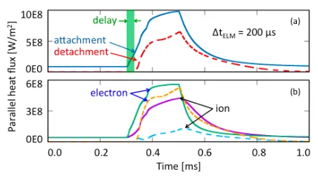
The heat flux to the target plate after an ELM crash in the detachment starts to increase with a delay of∼30µs, contrary to the sudden increase in the attachment in Fig. 2 (a). It is also found in Fig. 2 (b) that the difference between electron heat flux and ion heat flux to the plate becomes much larger in the detachment, while their heat fluxes are similar in the attachment. The above delay is caused by the transition process from detachment to attach-ment.
Because of the strong equipartition between ion and electron temperatures in detachment, the ion heat is trans-ferred to electrons before reaching the divertor plate as shown in Fig. 3, where the equipartition heat flux is the line integral from the source region to the target for equiparti-tion power densityQeq=3(me/mi)n(Ti−Te)/τe. Therefore, the ion heat flux to the target is reduced.
3.1.1 Reverse flow in detachment
de-Fig. 2 (a) Comparison of time development of total parallel heat fluxes in attachment and detachment. (b) Ion and electron heat fluxes included in total heat fluxes. Solid and dashed lines represent attachment and detachment, respectively.
Fig. 3 Comparison of time developments of parallel heat flux of equipartition for attachment (solid line) and detachment (dashed line). Ion heat is transferred to electrons before reaching the divertor plate (right schematic).
tachment, we varyrimp from 0.5 % to 1.5 % to investigate the characteristics of reverse flow. As shown in Fig. 4 (a) att−t0 =0µs, the flow velocity in front of the target (s
=43 - 44 m) becomes smaller when we raiserimp. As time passes after ELM, the magnitude of reverse flow for higher
rimpbecomes larger and the peak of reverse flow leaves far-ther away from the target, even reaches to an upper stream above x point as seen in Figs. 4 (b) att−t0=50µs and (c) att−t0=100µs.
For the details, we investigate the spatial distribution of plasma pressurePi+Pe, densityneand ion temperature
Tiand electron temperatureTeas shown in Fig. 5. Here, we consider that the ion and electron temperatures rise quickly due to ELM, the plasma pressure in front of the target be-comes extremely high, and then the plasma flow is reversed to the upstream.
3.2
Grassy ELMs
We investigate grassy ELMs with smaller amplitude. Parameters of ELM arePgrassy=3.3 MW∼0.1Ptype I ELM, Γgrassy =1.48 × 10²²/s ∼ 0.15 Γtype I ELM, and Δt
ELM = 200µs. At first, we put two ELM pulses with 13 ms inter-val, and confirm that the repetition of the heat flux form at the target is realized in this model as shown in Fig. 6. Next, we put five ELM pulses with frequency fgrassy=2000 Hz into attachment and detachment as shown in Fig. 7. We find that the difference of ELM heat fluxes between
attach-Fig. 4 Spatial distribution of flow velocity at (a) 0µs after an ELM occurs in detachment, (b) 50µs and (c) 100µs. Pur-ple and green lines represent cases ofrimp =0.5 % and
1.5 %, respectively.
Fig. 5 Temporal change of spatial distributions after an ELM in detachment (solid, dotted and dashed lines represent the line t−t0 =0µs, 50µs, and 100µs, respectively): (a)
plasma pressure, Pi+Pe, for the range s=39 - 44 m.
(b) densityne, ion temperatureTi, and electron
temper-atureTenear the targets=43 - 44 m for the case ofrimp
=1.5 %.
ment and detachment in grassy ELM case is much larger than that in type I ELM case. It implies that detached plasma is effective in lower power of ELM. On the other hand, we find a compound phenomenon of the accumula-tion of heat flux between the first ELM pulse and the sec-ond pulse in detachment. The secsec-ond peak of the heat flux becomes higher than the first one.
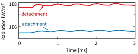
These dynamic responses are strongly dominated by the radiation effect. Figure 8 shows the difference in ra-diation heat flux between for detachment and for attach-ment, where the radiation heat flux is the line integral from the source region to the target for radiation power density
Qe,rad. Radiation power in detachment is higher by two
or-der than that in attachment all the time.
3.2.1 Radiation effect in detachment
In the above simulations, we adopt a simple radiative cooling model (Model I),Qe,rad =Lz(Te)nzne, and assume that the profile of impurity density is unchanged by the ELM pulse;nz(s) = nz(s,t = t0) = rimpne(s,t = t0) at
ef-Fig. 6 Repetition of parallel heat flux in detachment for two grassy ELM pulses with 13 ms interval.
Fig. 7 Time development of parallel heat flux in attachment (blue line) and detachment (red line) for five grassy ELM pulses withfgrassy=2000 Hz.
Fig. 8 Time development of parallel heat flux of radiation in at-tachment (blue line) and deat-tachment (red line).
fect (neτrecycle∼1015s·m−3).
Now we examine the sensitivity on the radiation model. We introduce another simple radiative cooling model (Model II),Qe,rad=Lz(Te)rimpn2e, where we assume that the impurity fractionrimp =1 % is kept constant and the impurity density is varied much by the ELM pulse;
nz(s, t) = rimpne(s, t). We find in attachment case as shown by Fig. 9 (a) that the amounts of ELM heat fluxes for Model II become smaller than that for Model I. On the other hand in detachment case as shown by Fig. 9 (b), first and second ELM-pulse heat fluxes for Model II are larger than those for Model I. After the third ELM-pulse, the heat flux for Model II decreases more rapidly than that for Model I. Figure 10 shows the radiation flux in detach-ment. The radiation flux for Model II is smaller than that for Model I at the beginning, but becomes larger than that for Model I in the end.
In addition to the impurity density response, the ELM pulse can affect the impurity recycling and resultantly
af-Fig. 9 Time development of parallel heat flux in (a) attachment and (b) detachment. Green and purple lines represent the cases of Model I (unchangednz) and Model II (constant
rimp), respectively.
Fig. 10 Time development of radiation flux in detachment. Green and purple lines represent the cases of Model I and Model II, respectively.
fect Lz(Te). Improvement in the radiation model for the precise analysis is a future work.
4. Conclusion
[1] A. Loarteet al., Nucl. Fusion47, S203 (2007). [2] N. Ohno, J. Plasma Fusion Res.92, 877 (2016). [3] S. Togoet al., Contrib. Plasma Phys.56, 729 (2016). [4] H. Uranoet al., Plasma Phys. Control. Fusion 45, 1571
(2003).
[5] B.N. Rogerset al., Phys. Rev. Lett.81, 4396 (1998).
[6] M. Sugiharaet al., Plasma Phys. Control. Fusion45, L55 (2003).
[7] S.I. Braginskii Reviews of Plasma Physics vol.1, p.205 (Consultants Bureau, New York, 1965).