SOFTWARE ARTICLE
K
ohdista
: an efficient method to index
and query possible Rmap alignments
Martin D. Muggli
1, Simon J. Puglisi
2and Christina Boucher
3*Abstract
Background: Genome-wide optical maps are ordered high-resolution restriction maps that give the position of occurrence of restriction cut sites corresponding to one or more restriction enzymes. These genome-wide optical maps are assembled using an overlap-layout-consensus approach using raw optical map data, which are referred to as Rmaps. Due to the high error-rate of Rmap data, finding the overlap between Rmaps remains challenging.
Results: We present Kohdista, which is an index-based algorithm for finding pairwise alignments between single molecule maps (Rmaps). The novelty of our approach is the formulation of the alignment problem as automaton path matching, and the application of modern index-based data structures. In particular, we combine the use of the Gen-eralized Compressed Suffix Array (GCSA) index with the wavelet tree in order to build Kohdista. We validate Kohdista on simulated E. coli data, showing the approach successfully finds alignments between Rmaps simulated from overlap-ping genomic regions.
Conclusion: we demonstrate Kohdista is the only method that is capable of finding a significant number of high qual-ity pairwise Rmap alignments for large eukaryote organisms in reasonable time.
Keywords: Optical mapping, Index based data structures, FM-index, Graph algorithms
© The Author(s) 2019. This article is distributed under the terms of the Creative Commons Attribution 4.0 International License (http://creat iveco mmons .org/licen ses/by/4.0/), which permits unrestricted use, distribution, and reproduction in any medium, provided you give appropriate credit to the original author(s) and the source, provide a link to the Creative Commons license, and indicate if changes were made. The Creative Commons Public Domain Dedication waiver (http://creativecommons.org/ publicdomain/zero/1.0/) applies to the data made available in this article, unless otherwise stated.
Background
There is a current resurgence in generating diverse types of data, to be used alone or in concert with short read data, in order to overcome the limitations of short read data. Data from an optical mapping system [1] is one such example and has itself become more practical with falling costs of high-throughput methods. For example, the current BioNano Genomics Irys System requires one week and $1000 USD to produce the Rmap data for an average size eukaryote genome, whereas, it required $100,000 and 6 months in 2009 [2]. These technological advances and the demonstrated utility of optical mapping in genome assembly [3–7] have driven several recent tool development efforts [8–10].
Genome-wide optical maps are ordered high-reso-lution restriction maps that give the position of occur-rence of restriction cut sites corresponding to one or more restriction enzymes. These genome-wide optical maps are assembled using an overlap-layout-consensus approach using raw optical map data, which are referred to as Rmaps. Hence, Rmaps are akin to reads in genome sequencing. In addition, to the the inaccuracies in the fragment sizes, there is the possibility of cut sites being spuriously added or deleted; which makes the problem of finding pairwise alignments between Rmaps challenging. To date, however, there is no efficient, non-proprietary method for finding pairwise alignments between Rmaps, which is the first step in assembling genome-wide maps.
Several existing methods are superficially applicable to Rmap pairwise alignments but all programs either strug-gle to scale to even moderate size genomes or require significant further adaptation to the problem. Several methods exhaustively evaluate all pairs of Rmaps using dynamic programming. One of these is the method of
Open Access
*Correspondence: [email protected]
3 Computer & Information Science & Engineering, University of Florida,
Gainesville, FL, USA
Valouev et al. [11], which is capable of solving the prob-lem exactly but requires over 100,000 CPU hours to com-pute the alignments for rice [12]. The others are SOMA [13] and MalignerDP [10] which are designed only for semi-global alignments instead of overlap alignments, which are required for assembly.
Other methods reduce the number of map pairs to be individually considered by initially finding seed matches and then extending them through more intensive work. These include OMBlast [9], OPTIMA [8], and Malign-erIX [10]. These, along with MalignerDP, were designed for a related alignment problem of aligning consensus data but cannot consistently find high quality Rmap pair-wise alignments in reasonable time as we show later. This is unsurprising since these methods were designed for either already assembled optical maps or in silico digested sequence data for one of their inputs, both having a lower error rate than Rmap data. In addition, Muggli et al. [14] presented a method called Twin, which aligns assembled contigs to a genome-wide optimal map. Twin varies from these previous methods in that it is unable to robustly find alignments between pairs of Rmaps due to the pres-ence of added or missing cut-sites.
In this paper, we present a fast, error-tolerant method for performing pairwise Rmap alignment that makes use of a novel FM-index based data structure. Although the FM-index can naturally be applied to short read align-ment [15, 16], it is nontrivial to apply it to Rmap align-ment. The difficulty arises from: (1) the abundance of missing or false cut sites, (2) the fragment sizes require inexact fragment-fragment matches (e.g. 1547 bp and 1503 bp represent the same fragment), (3) the Rmap sequence alphabet consists of all unique fragment sizes and is so extremely large (e.g., over 16,000 symbols for the goat genome). The second two challenges render inefficient the standard FM-index backward search algo-rithm, which excels at exact matching over small alpha-bets since each step of the algorithm extends the search for a query string by a single character c. If the alphabet is small (say DNA alphabet) then a search for other sym-bols of the alphabet other than c can be incorporated without much cost to the algorithm’s efficiency. Yet, if the alphabet is large enough this exhaustive search becomes impractical. The wavelet tree helps to remedy this prob-lem. It allows efficiently answering queries of the form: find all symbols that allow extension of the backward search by a single character, where the symbol is within the range [α1. . . αk] and where α1 and αk are symbols in
the alphabet such that α1≤αk [17]. In the case of
opti-cal mapping data, the alphabet is all fragment sizes. Thus, Muggli et al. [14] showed that constructing the FM-index and wavelet tree from this input can allow for sizing error to be account for by replacing each query in the FM index
backward search algorithm with a range query supported by the wavelet tree, i.e., if the fragment size in the query string is x then the wavelet tree can support queries of the form: find all fragment sizes that allow extension of the backward search by a single fragment, where the frag-ment size in the range [x−y,x+y] occur, where y is a
threshold on the error tolerance.
Muggli et al. [14] demonstrated that the addition of the wavelet tree can remedy the first two problems, i.e., sizing error and alphabet size, but the first and most-notable challenge requires a more complex index-based data structure. The addition of the wavelet tree to the FM-index is not enough to allow for searches that are robust to inserted and deleted cut sites. To overcome the challenge of having added or deleted cut sites while still accommodating the other two challenges, we develop Kohdista, an index-based Rmap alignment program that is capable of finding all pairwise alignments in large eukaryote organisms.
We first abstract the problem to that of approximate-path matching in a directed acyclic graph (DAG). The Kohdista method then indexes a set of Rmaps repre-sented as a DAG, using a modified form of the general-ized compressed suffix array (GCSA), which is a variant of the FM-index developed by Sirén et al. [18]. Hence, the constructed DAG, which is stored using the GCSA, stores all Rmaps, along with all variations obtained by considering all speculative added and deleted cut sites. The GCSA stores the DAG in a manner such that paths in DAG may be queried efficiently. If we contrast this to naïve automaton implementations, the GCSA has two advantages: it is space efficient, and it allows for efficient queries. Lastly, we demonstrate that challenges posed by the inexact fragment sizes and alphabet size can be over-come, specifically in the context of the GCSA, via careful use of a wavelet tree [17], and via using statistical criteria to control the quality of the discovered alignments.
Next, we point out some practical considerations con-cerning Kohdista. First, we note that Kohdista can be easily parallelized since once the GCSA is constructed from the Rmap data, it can be queried in parallel on as many threads as there are Rmaps to be queried. Next, in this paper, we focus on finding all pairwise alignments that satisfy some statistical constraints—whether they be global or local alignments. Partial alignments can be easily obtained by considering the prefix or suffix of the query Rmap and relaxing the statistical constraint.
larger eukaryote genomes by demonstrating that existing published methods require more than 151 h of CPU time to find all pairwise alignments in the plum Rmap data; whereas, Kohdista requires 31 h. Thus, we present the first fully-indexed method capable of finding all match patterns in the pairwise Rmap alignment problem.
Preliminaries and definitions
Throughout we consider a string (or sequence) S=S[1. . .n] =S[1]S[2]. . .S[n] of |S| =n symbols drawn from the alphabet [1. . . σ] . For i=1,. . .,n we
write S[i…n] to denote the suffix of S of length n−i+1 ,
that is S[i. . .n] =S[i]S[i+1]. . .S[n] , and S[1…i] to
denote the prefix of S of length i. S[i…j] is the sub-string S[i]S[i+1]. . .S[j] of S that starts at position i and ends at j. Given a sequence S[1, n] over an alpha-bet �= {1,. . .,σ} , a character c∈ , and integers i,j, rankc(S,i) is the number of times that c appears in S[1, i],
and selectc(S,j) is the position of the j-th occurrence of c
in S. We remove S from the functions when it is implicit from the context.
Overview of optical mapping
From a computer science viewpoint, restriction map-ping (by optical or other means) can be seen as a pro-cess that takes in two sequences: a genome A[1,n] and
a restriction enzyme’s restriction sequence B[1,b] , and
produces an array (sequence) of integers C , the genome restriction map, which we define as follows. First define the array of integers C[1,m] where C[i] =j if and only if A[j. . .j+b] =B is the ith occurrence of B in A .
Then R[i] =(C[i] −C[i−1]) , with R[1] =C[1] −1 .
In words, R contains the distance between
occur-rences of B in A . For example, if we let B be act and A=atacttactggactactaaact then we would have C=3, 7, 12, 15, 20 and R=2, 4, 5, 3, 5 . In reality, R is a
consensus sequence formed from millions of erroneous Rmap sequences. The optical mapping system produces millions of Rmaps for a single genome. It is performed on many cells of an organism and for each cell there are thousands of Rmaps (each at least 250 Kbp in length in publicly available data). The Rmaps are then assembled to produce a genome-wide optical map. Like the final R
sequence, each Rmap is an array of lengths—or fragment sizes—between occurrences of B in A.
There are three types of errors that an Rmap (and hence with lower magnitude and frequency, also the consensus map) can contain: (1) missing and false cuts, which are caused by an enzyme not cleaving at a specific site, or by random breaks in the DNA molecule, respec-tively; (2) missing fragments that are caused by desorp-tion, where small ( <1 Kbp ) fragments are lost and so
not detected by the imaging system; and (3) inaccuracy
in the fragment size due to varying fluorescent dye adhe-sion to the DNA and other limitations of the imaging process. Continuing again with the example above where
R=2, 4, 5, 3, 5 is the error-free Rmap: an example of an
Rmap with the first type of error could be R′=6, 5, 3, 5
(the first cut site is missing so the fragment sizes 2, and 4 are summed to become 6 in R′ ); an example of an Rmap
with the second type of error would be R′′=2, 4, 3, 5 (the
third fragment is missing); and lastly, the third type of error could be illustrated by R′′′=2, 4, 7, 3, 5 (the size of
the third fragment is inaccurately given).
Frequency of errors
In the optical mapping system, there is a 20% probability that a cut site is missed and a 0.15% probability of a false break per Kbp, i.e., error type (1) occurs in a fragment. Popular restriction enzymes in optical mapping experi-ments recognize a 6 bp sequence giving an expected cut-ting density of 1 per 4096 bp. At this cutcut-ting density, false breaks are less common than missing restriction sites (approx. 0.25∗.2=.05 for missing sites vs. 0.0015 for
false sites per bp). The error in the fragment size is nor-mally distributed with a mean of 0 bp, and a variance of
ℓσ2 , where ℓ is equal to the fragment length and σ =.58
kbp [11].
Suffix arrays, BWT and backward search
The suffix array [19] SAX (we drop subscripts when they are
clear from the context) of a sequence X is an array SA[1. . .n]
which contains a permutation of the integers [1...n] such that
X[SA[1]. . .n]<X[SA[2]. . .n]<· · ·<X[SA[n]. . .n].
In other words, SA[j] =i iff X[i. . .n] is the jth suffix of X in lexicographic order. For a sequence Y , the Y-interval in
the suffix array SAX is the interval SA[s. . .e] that contains
all suffixes having Y as a prefix. The Y-interval is a
represen-tation of the occurrences of Y in X . For a character c and a
sequence Y , the computation of cY-interval from Y-interval
is called a left extension.
The Burrows–Wheeler Transform BWT[1. . .n] is a permutation of X such that BWT[i] =X[SA[i] −1] if SA[i]>1 and $ otherwise [20]. We also define LF[i] =j
iff SA[j] =SA[i] −1 , except when SA[i] =1 , in which
case LF[i] =I , where SA[I] =n . Ferragina and
Man-zini [21] linked BWT and SA in the following way. Let
C[c] , for symbol c, be the number of symbols in X
lexi-cographically smaller than c. The function rank(X,c,i) ,
for sequence X , symbol c, and integer i, returns the
number of occurrences of c in X[1. . .i] . It is well known
that LF[i] =C[BWT[i]] +rank(BWT,BWT[i],i) .
the cY-interval. This is called backward search, and a data
structure supporting it is called an FM-index [21].
To support rank queries in backward search, a data structure called a wavelet tree can be used [17]. It occupies
nlogσ+o(nlogσ ) bits of space and supports rank
que-ries in O(logσ ) time. Wavelet trees also support a variety
of more complex queries on the underlying string effi-ciently. We refer the reader to Gagie et al. [17] for a more thorough discussion of wavelet trees. One such query we will use in this paper is to return the set X of distinct sym-bols occurring in S[i, j], which takes O(|X|logσ ) time.
The pairwise Rmap alignment problem
The pairwise Rmap alignment problem aims to align one Rmap (the query) Rq against the set of all other Rmaps
in the dataset (the target). We denote the target database as R1. . .Rn , where each Ri is a sequence of mi fragment
sizes, i.e, Ri= [fi1,. . .,fimi] . An alignment between two
Rmaps is a relation between them comprising groups of zero or more consecutive fragment sizes in one Rmap associated with groups of zero or more consecutive frag-ments in the other. For example, given Ri= [4, 5, 10, 9, 3]
and Rj= [10, 9, 11] one possible alignment is
{[4, 5],[10]},{[10],[9]},{[9],[11]},{[3],[]} . A group may
contain more than one fragment (e.g. [4, 5]) when the restriction site delimiting the fragments is absent in the corresponding group of the other Rmap (e.g [10]). This can occur if there is a false restriction site in one Rmap, or there is a missing restriction site in the other. Since we cannot tell from only two Rmaps which of these scenarios occurred, for the purpose of our remaining discussion it will be sufficient to consider only the scenario of missed (undigested) restriction sites.
Implementation
We now describe the algorithm behind Kohdista. Three main insights enable our index-based aligner for Rmap data: (1) abstraction of the alignment problem to a finite automaton; (2) use of the GCSA for storing and querying the automaton; and (3) modification of backward search to use a wavelet tree in specific ways to account for the Rmap error profile.
Finite automaton
Continuing with the example in the background section, we want to align R′=6, 5, 3, 5 to R′′′=2, 4, 7, 3, 5 and
vice versa. To accomplish this we cast the Rmap alignment problem to that of matching paths in a finite automaton. A finite automaton is a directed, labeled graph that defines a
language, or a specific set of sequences composed of ver-tex labels. A sequence is recognized by an automaton if it contains a matching path: a consecutive sequence of vertex
labels equal to the sequence. We represent the target Rmaps as an automaton and the query as a path in this context.
Backbone
The automaton for our target Rmaps can be constructed as follows. First, we concatenate the R1. . .Rn together
into a single sequence with each Rmap separated by a special symbol which will not match any query sym-bol. Let R∗ denote this concatenated sequence. Hence, R∗= [f11,. . .,f1m1,. . .,fn1,. . .,fnmn] . Then, construct an
initial finite automaton A=(V,E) for R∗ by creating
a set of vertices v1i. . .vim , one vertex per fragment for
a total of |R∗| vertices and each vertex is labeled with
the length its corresponding fragment. Edges are then added connecting vertices representing consecutive pairs of elements in R∗ . Also, introduce to A a starting vertexv1 labeled with # and a final vertexvf labeled with
the character $. All other vertices in A are labeled with
integral values. This initial set of vertices and edges is called the backbone. The backbone by itself is only sufficient for finding alignments with no missing cut sites in the query. The backbone of an automaton con-structed for a set containing R′ and R′′ would be #, 6, 5,
3, 5, 999, 2, 4, 3, 5$, using 999 as an unmatchable value. Next, extra vertices (“skip vertices”) and extra edges are added to A to allow for the automaton to accept all
valid queries. Figure 1a illustrates the construction of A
for a single Rmap with fragment sizes 2, 3, 4, 5, 6.
Skip vertices and skip edges
We introduce extra vertices labeled with compound
Generalized compressed suffix array
We index the automaton with the GCSA for efficient storage and path querying. The GCSA is a generaliza-tion of the FM-index for automata. We will explain the GCSA by drawing on the definition of the more widely-known FM-index. As stated in the background section, the FM-index is based on the deep relationship between the SA and the BWT data structures of the input string X . The BWT of an input string is formed by sorting all
characters of the string by the lexicographic order of the suffix immediately following each character. The
main properties the FM-index exploits in order to per-form queries efficiently are (a) BWT[i] =X[SA[i] −1] ;
and (b) given that SA[i] =j , and C[c] gives the position
of the first suffix in SA prefixed with character c, then
using small auxiliary data structures we can quickly determine k=C[BWT[i]] +rank(BWT,BWT[i],i) , such that SA[k] =j−1 . The first of these properties
is simply the definition of the BWT . The second is,
because the symbols of X occur in the same order in
both the single character prefixes in the suffix array and in the BWT , given a set of sorted suffixes, prepending
5,6,$ 5 4
4 3
3 2
2 #
#
6,$ 6
$ $ 7
7
11,$ 11
5 5
9,6,# 9
5,6,$ 5 4
4 3
3 2
2 #
#
6,$ 6
$ $ 7
7
11,$ 11
5,4 5
9,6,# 9
5,9,6,$ 5
a
b
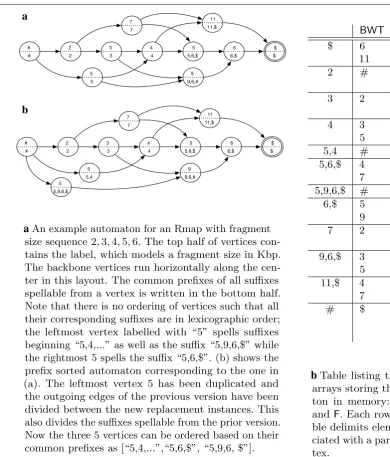
a An example automaton for an Rmap with fragment
size sequence 2,3,4,5,6. The top half of vertices con-tains the label, which models a fragment size in Kbp. The backbone vertices run horizontally along the cen-ter in this layout. The common prefixes of all suffixes spellable from a vertex is written in the bottom half. Note that there is no ordering of vertices such that all their corresponding suffixes are in lexicographic order; the leftmost vertex labelled with “5” spells suffixes beginning “5,4,...” as well as the suffix “5,9,6,$” while the rightmost 5 spells the suffix “5,6,$”. (b) shows the prefix sorted automaton corresponding to the one in (a). The leftmost vertex 5 has been duplicated and the outgoing edges of the previous version have been divided between the new replacement instances. This also divides the suffixes spellable from the prior version. Now the three 5 vertices can be ordered based on their common prefixes as [“5,4,...”,“5,6,$”, “5,9,6, $”].BWT M F
$ 6
11
1 1 0
2 # 1
0 1
3 2 1
0 1
4 3
5 10 10
5,4 # 1 1
5,6,$ 4 7
1 1 0 5,9,6,$ # 1 1
6,$ 5
9 1 10
7 2 1
0 1
9,6,$ 3
5 1 10 11,$ 4
7
1 1 0
# $ 1
0 0
1
b Table listing the three
arrays storing the automa-ton in memory: BWT, M, andF. Each row in the ta-ble delimits elements asso-ciated with a particular ver-tex.the same character onto each suffix does not change their order. Thus, if we consider all the suffixes in a range of SA which are preceded by the same symbol c,
that subset will appear in the same relative order in SA :
as a contiguous subinterval of the interval that contains all the suffixes beginning with c. Hence, by knowing where the position of the internal in SA corresponding
to a symbol, and the rank of an instance of that symbol,
we can identify the SA position beginning with that
instance from its position in BWT . A rank data
struc-ture over the BWT constitutes a sufficient compressed
index of the suffix array needed for traversal.
To generalize the FM-index to automata from strings, we need to efficiently store the vertices and edges in a manner such that the FM-index properties still hold, allowing the GCSA to support queries efficiently. An FM-index’s compressed suffix array for a string S encodes a relationship between each suffix S and its left extension. Hence, this suffix array can be generalized to edges in a graph that represent a relationship between vertices. The compressed suffix array for a string is a special case where the vertices are labeled with the string’s symbols in a non-branching path.
Prefix‑sorted automata
Just as backward search for strings is linked to suffix sort-ing, backward searching in the BWT of the automaton requires us to be able to sort the vertices (and a set of the paths) of the automaton in a particular way. This property is called prefix-sorted by Sirén et al. [18]. Let A=(V,E) be a finite automaton, let v|V| denote its terminal vertex, and let v∈V be a vertex. We say v is prefix-sorted by prefix p(v)
if the labels of all paths from v to v|V| share a common prefix p(v), and no path from any other vertex u =v to v|V| has p(v) as a prefix of its label. Automaton A is prefix-sorted if all vertices are prefix-sorted. See Fig. 1a for an example of a non-prefix sorted automaton and a prefix sorted automa-ton. A non-prefix sorted automaton can be made prefix sorted through a process of duplicating vertices and their incoming edges but dividing their outgoing edges between the new instances. We refer the reader to Sirén et al. [18]) for a more thorough explanation of how to transform a non-prefix sorted automaton to a prefix-sorted one.
Clearly, the prefixes p(v) allow us to sort the vertices of a prefix-sorted automaton into lexicographical order. Moreover, if we consider the list of outgoing edges (u, v), sorted by pairs (p(u), p(v)), they are also sorted by the sequences ℓ(u)p(v) , where ℓ(u) denotes the label of
ver-tex u. This dual sortedness property allows backward searching to work over the list of vertex labels (sorted by p(v)) in the same way that is does for the symbols of a string ordered by their following suffixes in normal back-ward search for strings.
Each vertex has a set of one or more preceding vertices and therefore, a set of predecessor labels in the automa-ton. These predecessor label sets are concatenated to form the BWT . The sets are concatenated in the order
defined by the above mentioned lexicographic ordering of the vertices. Each element in BWT then denotes an edge
in the automaton. Another bit vector, F , marks a ‘1’ for the first element of BWT corresponding to a vertex and a ‘0’
for all subsequent elements in that set. Thus, the prede-cessor labels, and hence the associated edges, for a vertex with rank r are BWT[select1(F,r) . . .select1(F,r+1)] . Another array, M , stores the outdegree of each vertex and allows the set of vertex ranks associated with a BWT interval to be found using rank() queries.
Exact matching: GCSA backward search
Exact matching with the GCSA is similar to the standard FM-index backward search algorithm. As outlined in the background section, FM-index backward search proceeds by finding a succession of lexicographic ranges that match progressively longer suffixes of the query string, start-ing from the rightmost symbol of the query. The search maintains two items—a lexicographic range and an index into the query string—and the property that the path pre-fix associated with the lexicographic range is equal to the suffix of the query marked by the query index. Initially, the query index is at the rightmost symbol and the range is [1…n] since every path prefix matches the empty suf-fix. The search continues using GCSA’s backward search step function, which takes as parameters the next symbol (to the left) in the query (i.e. fragment size in Rq ) and the
current range, and returns a new range. The query index is advanced leftward after each backward search step. In theory, since the current range corresponds to a consec-utive range in the BWT , the backward search could use select() queries on the bit vector F (see above) to
deter-mine all the edges adjacent to a given vertex and then two FM-index LF() queries are applied to the limits of the
current range to obtain the new one. GCSA’s implemen-tation uses one succinct bit vector per alphabet symbol to encode which symbols precede a given vertex instead of F . Finally, this new range, which corresponds to a set of edges, is mapped back to a set of vertices using rank() on the M bit vector.
backtracking to allow aligning Rmaps in the presence of multiple alternative size substitutions candidates as well as alternative compound fragments for each point in the query. We now discuss these modifications in further detail below.
To accommodate possible false restriction sites that are present in the query Rmap, we generate compound frag-ments by summing pairs and triples of consecutive query fragment sizes. This summing of multiple consecutive query fragments is complementary to the skip vertices in the target automaton which accommodate false restric-tion sites in the target. We note for each query Rmap there will be multiple combinations of compound frag-ments generated.
Next, in order to accommodate possible sizing error in the Rmap data, we modified the backward search by add-ing and usadd-ing a wavelet tree in our query of the GCSA. The original implementation of the GCSA does not con-struct or use the wavelet tree. Although it does consider alignments containing mismatches, it is limited to small alphabets (e.g., DNA alphabet), which do not necessitate the use of the wavelet tree. Here, the alphabet size is all possible fragment sizes. Thus, we construct the wavelet tree in addition to the GCSA. Then when aligning frag-ment f in the query Rmap, we determine the set of candi-date fragment sizes that are within some error tolerance of f by enumerating the distinct symbols in the currently active backward search range of the BWT using the
wave-let tree algorithm of Gagie et al. [17]. As previously men-tioned, this use of the wavelet tree also exists in the Twin [14] but is constructed and used in conjunction with an FM-index. We used the SDSL-Lite library by Gog et al. [22] to construct and store the GCSA.
Finally, since there may be multiple alternative size compatible candidates in the BWT interval of R∗ for
a compound fragment and multiple alternative com-pound fragments generated at a given position in query Rmap, we add backtracking to backward search so each candidate alignment is evaluated. We note that this is akin to the use of backtracking algorithms in short read alignment [15, 16]. Thus, for a given compound frag-ment size f generated from Rq , every possible candidate
fragment size, f′ , that can be found in R∗ in the range
f −t. . .f +t and in the interval s. . .e (of the BWT of R∗ ) for some tolerance t is considered as a possible
sub-stitute in the backward search.
Thus, to recap, when attempting to align each query Rmap, we consider every possible combination of com-pound fragments and use the wavelet tree to determine possible candidate matches during the backward search. There are potentially a large number of possible can-didate alignments—for efficiency, these cancan-didates are pruned by evaluating the alignment during each step of
the search relative to statistical models of the expected error in the data. We discuss this pruning in the next subsection.
Pruning the search
Alignments are found by incrementally extending can-didate partial alignments (paths in the automaton) to longer partial alignments by choosing one of several compatible extension matches (adjacent vertices to the end of a path in the automaton). To perform this search efficiently, we prune the search by computing the Chi-squared CDF and binomial CDF statistics of the partial matches and use thresholds to ensure reasonable size agreement of the matched compound fragments, and the frequency of putative missing cut sites. We conclude this section by giving an example of the backward search.
Size agreement
We use the Chi-squared CDF statistic to assess size agreement. This assumes the fragment size errors are independent, normally distributed events. For each pair of matched compound fragments in a partial alignment, we take the mean between the two as the assumed true length and compute the expected standard deviation using this mean. Each compound fragment deviates from the assumed true value by half the distance between them. These two values contribute two degrees of free-dom to the Chi-squared calculation. Thus, each devia-tion is normalized by dividing by the expected standard deviation, these are squared, and summed across all compound fragments to generate the Chi-squared sta-tistic. We use the standard Chi-squared CDF function to compute the area under the curve of the probability mass function up to this Chi-squared statistic, which gives the probability two Rmap segments from common genomic origin would have a Chi-squared statistic no more extreme than observed. This probability is
com-pared to Kohdista’s chi-squared-cdf-thresh and
if smaller, the candidate compound fragment is assumed to be a reasonable match and the search continues.
Cut site error frequency
above, this gives the probability two Rmaps of common genomic origin would have the number of non-conserved sites seen or fewer in the candidate partial alignment under consideration. This is compared to the binom-cdf-thresh to decide whether to consider extensions to the given candidate partial alignment. Thus, given a set of
Rmaps and input parameters binom-cdf-thresh and
chi-squared-cdf-thresh, we produce the set of all Rmap alignments that have a Chi-squared CDF statistic
less than chi-squared-cdf-thresh and a binomial
CDF statistic less than binom-cdf-thresh. Both of
these are subject to the additional constraint of a maxi-mum consecutive missed restriction site run between aligned sites of two and a minimum aligned site set car-dinality of 16.
Example traversal
A partial search for a query Rmap [3 kb, 7 kb, 6 kb] in Fig. 1a and Table (b) given an error model with a constant 1 kb sizing error would proceed with steps:
1. Start with the semi-open interval matching the empty string [0…12).
2. A wavelet tree query on BWT would indicate the set of symbols {5, 6, 7} is the intersection of two sets: (a) the set of symbols that would all be valid left exten-sions of the (currently empty) match string and (b) the set of size appropriate symbols that match our next query symbol (i.e. 6 kb, working from the right end of our query) in light of the expected sizing error (i.e. 6kb +/− 1 kb).
3. We would then do a GCSA backward search step on the first value in the set (5) which would yield the new interval [4…7). This new interval denotes only nodes where each node’s common prefix is compat-ible with the spelling of our current backward tra-versal path through the automaton (i.e. our short path of just [5] does not contradict any path spella-ble from any of the three nodes denoted in the match interval).
4. A wavelet tree query on the BWT for this interval for values 7 kb +/− 1 kb would return the set of symbols {7}.
5. Another backward search step would yield the new interval [8…9). At this point our traversal path would be [7, 5] (denoted as a left extension of a forward path that we are building by traversing the graph backward). The common prefix of each node (only one node here) in our match interval (i.e. [7 kb]) is compatible with the path [7, 5]. This process would continue until backward search returns no match
interval or our scoring model indicates our repeat-edly left extended path has grown too divergent from our query. At this point backtracking would occur to find other matches (e.g. at some point we would backward search using the value 6 kb instead of the 5 kb obtained in step 2.)
Practical considerations
In this section we describe some of the practical consid-erations that were made in the implementation.
Memoization
One side effect of summing consecutive fragments in both the search algorithm and the target data structure is that several successive search steps with agreeing frag-ment sizes will also have agreeing sums of those succes-sive fragments. In this scenario, proceeding deeper in the search space will result in wasted effort. To reduce this risk, we maintain a table of scores obtained when reaching a particular lexicographic range and query cur-sor pair. We only proceed with the search past this point when either the point has never been reached before, or has only been reached before with inferior scores.
Wavelet tree threshold
The wavelet tree allows efficiently finding the set of ver-tex labels that are predecessors of the vertices in the current match interval intersected with the set of vertex labels that would be compatible with the next compound fragment to be matched in the query. However, when the match interval is sufficiently small ( <750 ) it is faster to scan the vertices in BWT directly.
Quantization
The alphabet of fragment sizes can be large considering all the measured fragments from multiple copies of the genome. This can cause an extremely large branching factor for the initial symbol and first few extensions in the search. To improve the efficiency of the search, the fragment sizes are initially quantized, thus reducing the size of the effective alphabet and the number of substitu-tion candidates under considerasubstitu-tion at each point in the search. Quantization also increases the number of identi-cal path segments across the indexed graph which allows a greater amount of candidate matches to be evaluated in parallel because they all fall into the same BWT interval
Results
We evaluated Kohdista against the other available opti-cal map alignment software. Our experiments measured runtime, peak memory, and alignment quality on simu-lated E. coli Rmaps and experimentally generated plum Rmaps. All experiments were performed on Intel Xeon computers with ≥ 16 GB RAM running 64-bit Linux.
Parameters used We tried OPTIMA with both “p-value” and “score” scoring and the allMaps option and report the higher sensitivity “score” setting. We followed the OPTIMA-Overlap protocol of splitting Rmaps into
k-mers, each containing 12 fragments as suggested in [8]. For OMBlast, we adjusted parameters maxclusteritem, match, fpp, fnp, meas, minclusterscore, and minconf. For MalignerDP, we adjusted parameters max-misses, miss-penalty, sd-rate, min-sd, and max-miss-rate and addi-tionally filtered the results by alignment score. Though unpublished, for comparison we also include the propri-etary RefAligner software from BioNano. For RefAligner we adjusted parameters FP, FN, sd, sf, A, and S. For
Koh-dista, we adjusted parameters
chi-squared-cdf-thresh and binom-cdf-thresh. For the method of Valouev et al. [12], we adjusted score_thresh and t_score_ thresh variables in the source. In Table 1 we report sta-tistical and computational performance for each method.
OMBlast was configured with parameters meas =
3000, minconf = 0.09, minmatch = 15 and the rest left at
defaults. RefAligner was run with parameters FP = 0.15,
sd = 0.6, sf = 0.2, sr = 0.0, se = 0.0, A = 15, S = 22 and
the rest left at defaults. MalignerDP was configured with parameters ref-max-misses = 2, query-miss-penalty = 3,
query-max-miss-rate = 0.5, min-sd = 1500, and the rest
left at defaults.
The method of Valouev et al. [12] was run with default parameters except we reduced the maximum compound fragment length (their δ parameter) from 6 fragments to
3. We observed this method rarely included alignments containing more than two missed restriction sites in a compound fragment.
Performance on simulated E. coli Rmap data
To verify the correctness of our method, we simulated a read set from a 4.6 Mbp E. coli reference genome as fol-lows: we started with 1,400 copies of the genome, and then generated 40 random loci within each. These loci form the ends of molecules that would undergo digestion. Molecules smaller than 250 Kbp were discarded, leav-ing 272 Rmaps with a combined length equatleav-ing to 35x coverage depth. The cleavage sites for the XhoI enzyme were then identified within each of these simulated mol-ecules. We removed 20% of these at random from each simulated molecule to model partial digestion. Finally, normally distributed noise was added to each fragment with a standard deviation of .58 kb per 1 kb of the frag-ment. This simulation resulted in 272 Rmaps. Simulated molecule pairs having 16 common conserved digestion sites become the set of “ground truth” alignments, which our method and other methods should successfully iden-tify. Our simulation resulted in 4,305 ground truth align-ments matching this criteria. Although a molecule would align to itself, these are not included in the ground truth set. This method of simulation was based on the E. coli
statistics given by Valouev et al. [12] and resulting in a molecule length distribution as observed in publicly available Rmap data from OpGen, Inc.
Most methods were designed for less noisy data but in theory could address all the data error types required. For methods with tunable parameters, we tried aligning the E. coli Rmaps with combinations of parameters for each method related to its alignment score thresholds and error model parameters. We used parameterization giving results similar to those for the default parameters of the method of Valouev et al. [12] to the extent such parameters did not significantly increase the running time of each method. These same parameterization were used in the next section on plum data.
Even with tuning, we were unable to obtain pair-wise alignments on E. coli for two methods. We found OPTIMA only produced self alignments with its
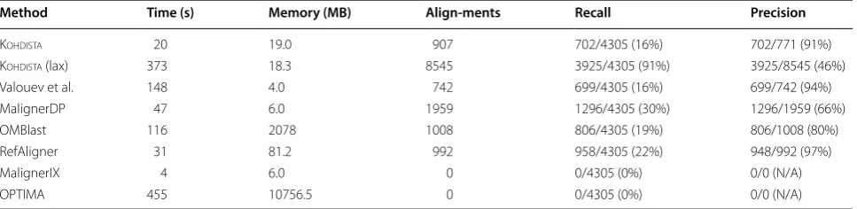
Table 1 Performance on simulated E. coli dataset
Kohdista (lax) demonstrates that our indexing and search method is capable of finding the majority of ground truth alignments when the search is pruned to the more
relaxed thresholds for chi-squared-cdf-thresh and binom-cdf-thresh, i.e., chi-squared-cdf-thresh= 0.02 and binom-cdf-thresh= 0.5
Method Time (s) Memory (MB) Align-ments Recall Precision
Kohdista 20 19.0 907 702/4305 (16%) 702/771 (91%)
Kohdista (lax) 373 18.3 8545 3925/4305 (91%) 3925/8545 (46%)
Valouev et al. 148 4.0 742 699/4305 (16%) 699/742 (94%)
MalignerDP 47 6.0 1959 1296/4305 (30%) 1296/1959 (66%)
OMBlast 116 2078 1008 806/4305 (19%) 806/1008 (80%)
RefAligner 31 81.2 992 958/4305 (22%) 948/992 (97%)
MalignerIX 4 6.0 0 0/4305 (0%) 0/0 (N/A)
recommended overlap protocol and report its resource use in Table 1. For MalignerIX, even when we relaxed the parameters to account for the greater sizing error and mismatch cut site frequency, it was also only able to find self alignments. This is expected as by design it only allows missing sites in one sequence in order to run faster. Thus no further testing was performed with
MalignerIX or OPTIMA. We did not test SOMA [13] as
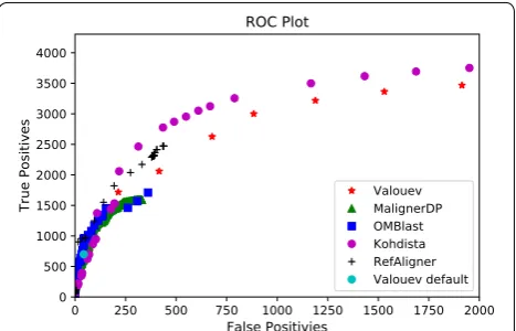
earlier investigation indicate it would not scale to larger genomes [14]. We omitted TWIN [14] as it needs all cut sites to match. With tuning, Kohdista, MAligner, the method of Valouev et al. [12], RefAligner and OMBlast produced reasonable results on the E.coli data. Results for the best combinations of parameters encountered during tuning can be seen in Figs. 2 and 3. We observed that most methods could find more ground truth align-ments as their parameters were relaxed at the expense of additional false positives, as illustrated in these figures. However, only the method of Valouev et al. and Koh-dista approached recall of all ground truth alignments.
Table 1 illustrates the results for Kohdista and the competing methods with parameters optimized to try to match those of Valouev et al. [12], as well as results using Kohdista with a more permissive parameter set-ting. All results include both indexing as well as search time. Kohdista took two seconds to build its data struc-tures. Again, Kohdista uses Chi-squared and binomial CDF thresholds to prune the backtracking search when deciding whether to extend alignments to progres-sively longer alignments. More permissive match crite-ria, using higher thresholds, allows more Rmaps to be reached in the search and thus to be considered aligned, but it also results in less aggressive pruning in the search, thus lengthening runtime. As an example, note that when Kohdista was configured with a much relaxed Chi-squared CDF threshold of .5 and a binomial CDF threshold of .7, it found 3925 of the 4305 (91%) ground truth alignments, but slowed down considerably. This
illustrates the index and algorithm’s capability in han-dling all error types and achieving high recall.
Performance on plum Rmap data
The Beijing Forestry University and other institutes assembled the first plum (Prunus mume) genome using short reads and optical mapping data from OpGen Inc. We test the various available alignment methods on the 139,281 plum Rmaps from June 2011 available in the GigaScience repository. These Rmaps were created with the BamHI enzyme and have a coverage depth of 135x of the 280 Mbp genome. For the plum dataset, we ran all the methods which approach the statistical performance of the method of Valouev et al. [12] when measured on E. coli. Thus, we omitted MalignerIX and OPTIMA because they had 0% recall and precision on E. coli. Our results on this plum dataset are summarized in Table 2.
Kohdista was the fastest and obtained more align-ments than the competing methods. When configured with the Chi-squared CDF threshold of .02 and binomial CDF threshold of .5, it took 31 h of CPU time to test all Rmaps for pairwise alignments in the plum Rmap data. This represents a 21× speed-up over the 678 h taken by the dynamic programming method of Valouev et al. [12]. MalignerDP and OMBlast took 214 h and 151 h, respec-tively. Hence, Kohdista has a 6.9× and 4.8× speed-up over MalignerDP and OMBlast. All methods used less
Fig. 2 Precision-recall plot of successful methods on simulated E. coli
Fig. 3 ROC plot of successful methods on simulated E. coli
Table 2 Performance on plum
Method Time (h) Memory Alignments
Kohdista 31 7.4 GB 16,109,151
Valouev et al. 678 60 MB 6387
MalignerDP 214 784 MB 1,258,328
OMBlast 151 12.3 GB 424,730
than 13 GB of RAM and thus, were considered practical from a memory perspective. Kohdista took 11 min to build its data structures for Plum.
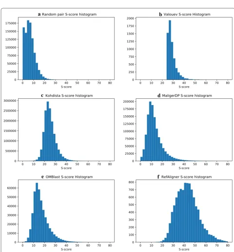
To measure the quality of the alignments, we scored each pairwise alignment using Valouev et al. [12] and presented histograms of these alignment scores in Fig. 4.
a
b
c
d
e
f
For comparison, we also scored and present the histo-gram for random pairs of Rmaps. The method of Valouev et al. [12] produces very few but high-scoring alignments and although it could theoretically be altered to pro-duce a larger number of alignments, the running time makes this prospect impractical (678 h). Although Koh-dista and RefAligner produce high-quality alignments, RefAligner produced very few alignments (10,039) and required almost 5x more time to do so. OMBlast and Maligner required significantly more time and produced significantly lower quality alignments.
Conclusions
In this paper, we demonstrate how finding pairwise align-ments in Rmap data can be modelled as approximate-path matching in a directed acyclic graph, and combining the GCSA with the wavelet tree results in an index-based data structure for solving this problem. We implement this method and present results comparing Kohdista with competing methods. By demonstrating results on both simulated E. coli Rmap data and real plum Rmaps, we show that Kohdista is capable of detecting high scoring alignments in efficient time. In particular, Koh-dista detected the largest number of alignments in 31 h. RefAligner, a proprietary method, produced very few high scoring alignments (10,039) and requires almost 5× more time to do so. OMBlast and Maligner required
significantly more time and produced significantly lower quality alignments. The method of Valouev et al. [12] produced high scoring alignments but required more than 21× time to do.
Availability and requirements Project name: Kohdista.
Project home page: https ://githu b.com/mmugg li/KOHDI STA.
Operating system(s): Developed for 32-bit and 64-bit Linux/Unix environments.
Programming language: C/C++. Other requirements: GCC 4.2 or newer. License: MIT license.
Any restrictions to use by non-academics: Non-needed.
Abbreviations
DAG: directed acyclic graph (DAG); SA: suffix array; GCSA: generalized com-pressed suffix array; BWT: Burrows–Wheeler Transform.
Acknowledgements
The authors would like to thank Jouni Sirén for many insightful conversations concerning the GCSA.
Authors’ contributions
SJP, MDM, and CB conceived of the concept and designed the algorithm and data structures for the methods described in this paper. MDM and CB designed the experiments. MDM implemented the method, and performed all experiments and software testing. MDM and CB drafted the manuscript. All authors read and edited the manuscript. All authors read and approved the final manuscript.
Funding
MDM, SJP, and CB were funded by the National Science Foundation (1618814). SJP was also supported in part by the Academy of Finland via Grant Number 294143.
Availability of data and materials
Kohdista is available at https ://githu b.com/mmugg li/KOHDI STA/. No original data was acquired for this research. The simulated E.coli data generated and analysed during the current study are available at https ://githu b.com/mmugg li/KOHDI STA. The plum (Prunus mume) dataset used in this research was acquired from the GigaScience repository http://gigad b.org/datas et/view/ id/10008 4/File_sort/size.
Ethics approval and consent to participate Not applicable.
Consent for publication Not applicable.
Competing interests
The authors declare that they have no competing interests.
Author details
1 Department of Computer Science, Colorado State University, Fort Collins,
CO, USA. 2 Department of Computer Science, University of Helsinki, Helsinki,
Finland. 3 Computer & Information Science & Engineering, University of Florida,
Gainesville, FL, USA.
Received: 1 November 2018 Accepted: 19 November 2019
References
1. Dimalanta ET, Lim A, Runnheim R, Lamers C, Churas C, Forrest DK, de Pablo JJ, Graham MD, Coppersmith SN, Goldstein S, Schwartz DC. A microfluidic system for large DNA molecule arrays. Anal Chem. 2004;76(18):5293–301.
2. Bionano Genomics Ilc. Bionano Genomics Launches Irys, a novel platform for complex human genome analysis; 2012. https ://biona nogen omics .com/press -relea ses/biona no-genom ics-launc hes-irys-a-novel -platf orm-for-compl ex-human -genom e-analy sis/.
3. Reslewic S, et al. Whole-genome shotgun optical mapping of Rhodospiril-lum rubrum. Appl Environ Microbiol. 2005;71(9):5511–22.
4. Zhou S, et al. A whole-genome shotgun optical map of Yersinia pestis strain KIM. Appl Environ Microbiol. 2002;68(12):6321–31.
5. Zhou S, et al. Shotgun optical mapping of the entire Leishmania major Friedlin genome. Mol Biochem Parasitol. 2004;138(1):97–106. 6. Chamala S, et al. Assembly and validation of the genome of the
non-model basal angiosperm amborella. Science. 2013;342(6165):1516–7. 7. Dong Y, et al. Sequencing and automated whole-genome optical
map-ping of the genome of a domestic goat ( capra hircus). Nat Biotechnol. 2013;31(2):136–41.
8. Verzotto D, et al. Optima: sensitive and accurate whole-genome align-ment of error-prone genomic maps by combinatorial indexing and technology-agnostic statistical analysis. GigaScience. 2016;5(1):2. 9. Leung AK, Kwok T-P, Wan R, Xiao M, Kwok P-Y, Yip KY, Chan T-F. OMBlast:
alignment tool for optical mapping using a seed-and-extend approach. Bioinformatics. 2017;33(3):311–9.
10. Mendelowitz LM, Schwartz DC, Pop M. Maligner: a fast ordered restriction map aligner. Bioinformatics. 2016;32(7):1016–22.
•fast, convenient online submission •
thorough peer review by experienced researchers in your field • rapid publication on acceptance
• support for research data, including large and complex data types •
gold Open Access which fosters wider collaboration and increased citations maximum visibility for your research: over 100M website views per year •
At BMC, research is always in progress.
Learn more biomedcentral.com/submissions
Ready to submit your research? Choose BMC and benefit from: 12. Valouev A, et al. An algorithm for assembly of ordered restriction maps
from single DNA molecules. Proc Natl Acad Sci. 2006;103(43):15770–5. 13. Nagarajan N, Read TD, Pop M. Scaffolding and validation of bacterial
genome assemblies using optical restriction maps. Bioinformatics. 2008;24(10):1229–35.
14. Muggli MD, Puglisi SJ, Boucher C. Efficient indexed alignment of contigs to optical maps. In: Proceedings of the 14th workshop on algorithms in bioinformatics (WABI). Berlin: Springer; 2014. p. 68–81.
15. Li H, Durbin R. Fast and accurate short read alignment with Burrows– Wheeler transform. Bioinformatics. 2009;25(14):1754–60.
16. Langmead B, Trapnell C, Pop M, Salzberg SL. Ultrafast and memory-efficient alignment of short DNA sequences to the human genome. Genome Biol. 2009;10(3):25.
17. Gagie T, Navarro G, Puglisi SJ. New algorithms on wavelet trees and appli-cations to information retrieval. Theor Comput Sci. 2012;426/427:25–41. 18. Sirén J, Välimäki N, Mäkinen V. Indexing graphs for path queries with
applications in genome research. IEEE/ACM Trans Comput Biol Bioinfor-matics. 2014;11(2):375–88.
19. Manber U, Myers GW. Suffix arrays: a new method for on-line string searches. SIAM J Sci Comput. 1993;22(5):935–48.
20. Burrows M, Wheeler DJ. A block sorting lossless data compression algo-rithm. Technical Report 124, Digital Equipment Corporation, Palo Alto, California. 1994.
21. Ferragina P, Manzini G. Indexing compressed text. J ACM. 2005;52(4):552–81.
22. Gog S, Beller T, Moffat A, Petri M. From theory to practice: plug and play with succinct data structures. In: Proceedings of the 13th international symposium on experimental algorithms, (SEA). 2014. p. 326–37.
Publisher’s Note