Constructing majority-rule supertrees

R E S E A R C H

Open Access

Constructing majority-rule supertrees

Jianrong Dong

, David Fernández-Baca

, FR McMorris

Abstract

Background:Supertree methods combine the phylogenetic information from multiple partially-overlapping trees into a larger phylogenetic tree called a supertree. Several supertree construction methods have been proposed to date, but most of these are not designed with any specific properties in mind. Recently, Cotton and Wilkinson proposed extensions of the majority-rule consensus tree method to the supertree setting that inherit many of the appealing properties of the former.

Results:We study a variant of one of Cotton and Wilkinson’s methods, called majority-rule (+) supertrees. After

proving that a key underlying problem for constructing majority-rule (+) supertrees is NP-hard, we develop a polynomial-size exact integer linear programming formulation of the problem. We then present a data reduction heuristic that identifies smaller subproblems that can be solved independently. While this technique is not guaranteed to produce optimal solutions, it can achieve substantial problem-size reduction. Finally, we report on a computational study of our approach on various real data sets, including the 121-taxon, 7-tree Seabirds data set of Kennedy and Page.

Conclusions:The results indicate that our exact method is computationally feasible for moderately large inputs. For larger inputs, our data reduction heuristic makes it feasible to tackle problems that are well beyond the range of the basic integer programming approach. Comparisons between the results obtained by our heuristic and exact solutions indicate that the heuristic produces good answers. Our results also suggest that the majority-rule (+) approach, in both its basic form and with data reduction, yields biologically meaningful phylogenies.

Background

Introduction

A supertree method begins with a collection of phyloge-netic trees with possibly different leaf (taxon) sets, and assembles them into a larger phylogenetic tree, a super-tree, whose taxon set is the union of the taxon sets of the input trees. Interest in supertrees was sparked by Gordon’s paper [1]. Since then, particularly during the past decade, there has been a flurry of activity with many supertree methods proposed and studied from the algorithmic, theoretical, and biological points of view. The appeal of supertree synthesis is that it can combine disparate data to provide a high-level perspective that is harder to attain from individual trees. A recent example of the use of this approach is the species-level phylogeny of nearly all extant Mammalia constructed by Bininda-Emonds [2] from over 2,500 partial estimates. Several of the known supertree methods are reviewed in the book

edited by Bininda-Emonds [3] — more recent papers

with good bibliographies include [4,5]. There is still much debate about what specific properties should (can), or should not (cannot), be satisfied by supertree methods. Indeed, it is often a challenging problem to rigorously determine the properties of a supertree method that gives seemingly good results on data, but is heuristic.

The well-studied consensus tree problem can be viewed as the special case of the supertree problem where the input trees have identical leaf sets. Consensus methods in systematics date back to [6]; since then, many consensus methods have been designed. A good survey of these methods, their properties, and their interrelationships is given by Bryant [7], while the axio-matic approach and the motivation from the social

sciences is found in Day and McMorris’ book [8]. One

of the most widely used methods is the majority-rule consensus tree [9,10], which is the tree that contains the splits displayed by the majority of the input trees. Not only does this tree always exist, but it is also unique, * Correspondence: [email protected]; [email protected]

1_{Department of Computer Science, Iowa State University, Ames, IA 50011,} USA

can be efficiently constructed [11], and has the property of being amedian treerelative to the symmetric-differ-ence distance (also known as the Robinson-Foulds dis-tance [12,13]). That is, the majority-rule consensus tree is a tree whose total Robinson-Foulds distance to the input trees is minimum.

The appealing qualities of the majority-rule consensus method have made it attractive to try to extend the method to the supertree setting, while retaining as many of its good characteristics as possible. Cotton and Wilk-inson [14] were able to define two such extensions (despite some doubts about whether such an extension was possible [15]) and at least two additional ones have been studied since [16]. Here we study one of the latter variants, called graft-refine majority-rule (+) supertrees in [16], and here simply referred to asmajority-rule (+) supertrees. These supertrees satisfy certain desirable properties with respect to what information from the input trees, in the form of splits, is displayed by them (see the Preliminaries). The key idea in this method is to expand the input trees by grafting leaves onto them to produce trees over the same leaf set. The expansion is done so as to minimize the distance from the expanded trees to their median relative to the Robin-son-Foulds distance. The supertree returned is the strict consensus of the median trees with minimum distance to the expanded input trees; these median trees are calledoptimal candidate supertrees.

After showing that computing an optimal candidate supertree is NP-hard, we develop a characterization of these supertrees that allows us to formulate the problem as a polynomial-size integer linear program (ILP). We then describe an implementation that enables us to solve moderately large problems exactly. We show that, in practice, the majority-rule (+) supertree can be con-structed quickly once an optimal candidate supertree has been identified. Furthermore, we observe that the supertrees produced are similar to biologically reason-able trees, adding further justification to the majority-rule (+) approach.

In addition to the exact ILP formulation, we also introduce a data reduction heuristic that identifies

“reducible” sets of taxa. Informally, these are taxa that are clustered in the same way by all the input trees. By restricting the original profile to the taxa in any such set, we get a“satellite profile” that can be much smaller than the original one. At the same time, the original profile can be reduced by representing all the taxa in the set by a single supertaxon. A supertree for the origi-nal profile is obtained by solving each of these supertree problems independently and combining the answers. This approach allows us to tackle supertree problems that are well beyond the limits of the basic ILP method. Thus, whereas the latter allowed us to solve instances at

most 40 taxa, the former enabled us to handle the Sea-birds data set of Kennedy and Page [17], which as 121 taxa. While the data reduction technique is not guaran-teed to produce the same answers as the exact method, we present empirical evidence that it produces good results. Moreover, reducible sets often correspond to meaningful biological classification units that likely should be respected by any supertree.

We should mention that the supertree method most commonly used in practice is matrix representation with parsimony (MRP) [18,19]. MRP first encodes the input trees as incomplete binary characters, and then builds a maximum-parsimony tree for this data. The popularity of MRP is perhaps due to the widespread acceptance of the philosophy underlying parsimony approaches and the availability of excellent parsimony software (e.g., [20]). However, while parsimony is relatively easy to justify in the original tree-building problem (in which homoplasy represents additional assumptions of evolutionary changes) a justification for its use as a supertree construc-tion method is not quite as obvious. Perhaps the main cri-ticism of MRP, as well as other tree construction methods, is that it can produce unsupported groups [21,22]. The provable properties of majority-rule (+) supertrees [14,16] prevent such anomalies. There has been previous work on ILP in phylogenetics, much of it dealing with parsimony or its relative, compatibility [23-27]. Our work uses some of these ideas (especially those of [26]), but the context and the objective function are quite different. In particular, the need to handle all possible expansions of the input trees necessitates the introduction of new techniques.

Preliminaries

Basic definitions and notation

Our terminology largely follows [28]. Aphylogenetic tree is an unrooted leaf-labeled tree where every internal node has degree at least three. We will use“tree” and

“phylogenetic tree” interchangeably. The leaf set of a treeT is denoted byL(T).

Aprofileis a tuple of treesP= (t1,...,tk). EachtiinPis

called an input tree. Let L(P) = ∪iKL(ti), where K

denotes the set {1,...,k}. An input treetiisplenaryifL(ti)

=L(P). TreeTis asupertreefor profilePifL(T) =L(P). A split is a bipartition of a set. We write A|B to

denote the split whose parts are Aand B. The order

here does not matter, soA|Bis the same as B|A. Split A|Bisnontrivialif each ofAandBhas at least two ele-ments; otherwise it is trivial. SplitA|B extends another splitC|DifA⊇CandB⊇D, orA⊇DandB⊇C.

Phylogenetic treeT displayssplitA|Bif there is an edge inTwhose removal gives treesT1andT2such thatA⊆

displayed byTis denoted Spl(T). It is well known that the full splits ofTuniquely identifyT[[28], p. 44]. LetS ⊆L(T). Therestriction of T to S, denotedT|S, is the phy-logenetic tree with leaf setSsuch that

Spl( | )T S {AS B| S A B: | Spl( )T and |AS|,|B S| 1}.

LetT’be a phylogenetic tree such that S=L(T’)⊆L (T). Then,T displays T’if Spl(T’)⊆Spl(T|S).

A set of splits is compatible if there is a tree T that

displays them all. Tree T is compatible with a set of

splits  if there is a treeT’that displays Tand . LetT1andT2 be two phylogenetic trees over the same leaf set. The symmetric-difference distance, also known asRobinson-Foulds distance [13], betweenT1 and T2, denotedd(T1,T2), is defined as

d T T( ,_{1 2}) |Spl( ) \T₁ Spl(T₂))(Spl(T₂) \Spl( )) | .T₁ (1)

The majority splitsin a profile P = (t1,..., tk) are the

splits displayed by more than ₂k of the input trees. A majority plenary split is a plenary split that is also a majority split. Similarly, a majority partial splitis a par-tial split that is also a majority split.

Rootedphylogenetic trees can be viewed as a special case of unrooted trees. That is, we can view a profile of rooted trees as unrooted trees, all of which have a com-mon taxon called the root. Thus, in a split in a rooted tree, one of the two parts must contain the root; the part that does not contain the root is called acluster(or clade, or monophyletic group). All of the above concepts (eg., compatibility and distance), as well as those intro-duced in the rest of this paper, directly apply to rooted trees. However, we shall not elaborate on this here.

To close this section, we examine theconsensus

pro-blem, the special case of the supertree problem where

the profileP= (T1,...,Tk) consists of trees that have the

same leaf set. Thestrict consensus ofP is the tree that displays exactly the plenary splits present in every tree in the profile. The majority-rule consensus treeof P, denoted Maj(P), is the tree that displays all the majority plenary splits inP[10]. For any phylogeny Twith L(T) =L(P), define the distance fromT toP as dist(T, P) =

ΣiKd(T,Ti), where ddenotes the symmetric-difference

distance. AnyTwith leaf setL(P) that minimizes dist(T, P) is called amedian treefor P. It is known that Maj(P) is a median tree forP; indeed, it follows from [9] that Maj(P) is the strict consensus of the median trees forP. The (median)scoreofPis defined as s(P) = minT:L(T)=L

(P)dist(T,P). Thus,s(P) = dist(Maj(P),P).

Majority-rule (+) supertrees

Here we describe a variant (suggested by Bill Day) of one of Cotton and Wilkinson’s [14] extensions of major-ity-rule consensus to the supertree setting.

Thespanof an input tree t, denoted by〈t〉, is the set of all trees onL(P) that display t. The spanof a profile P = (t1,..., tk), denoted〈P〉, is the set of allk-tuplesR=

(T1,...,Tk), whereTi〈ti〉for eachiK. EachR〈P〉is

called a representative selection for P and Maj(R) is called acandidate supertree.

Anoptimal representative selectionis a representative selection Rwith minimum score s(R) over all R 〈P〉. We refer to Maj(R) as theoptimal candidate supertree

associated with R. The majority-rule (+) supertree of

profileP, denoted by Maj+(P), is the strict consensus of all the optimal candidate supertrees. We have shown elsewhere [16] that Maj+(P) satisfies the following appealing properties (originally conjectured by Cotton and Wilkinson).

(CW1) Maj+(P) displays all of the majority plenary splits inP.

(CW2) Maj+(P) is compatible with each majority par-tial split inP.

(CW3) Each split in Maj+(P) is compatible with a

majority of the trees inP.

(CW4) Every plenary split in Maj+(P) extends at least one input tree full split.

We should note that majority-rule (+) supertrees, as defined above, do not generalize majority-rule consen-sus. That is, when used in the consensus setting, Maj +

(P) is not, in general, the same as Maj(P). Nevertheless, majority-rule (+) consensus trees have a simple charac-terization that yields an efficient algorithm for comput-ing them (see Theorem 1 of the Methods).

The majority-rule (+) supertrees we study differ from other variants in the way the span of an input tree is defined. Cotton and Wilkinson originally defined the span of a treetas the set of all plenary binarytrees that displayt[14]. This version does not generalize majority-rule consensus and does not satisfy (CW4) [16]. In a more recent version, suggested by Wilkinson (personal communication), the span of tis the set of all plenary treesTsuch thatT|L(t) =t. This definition of span pro-hibits refinement of any original polytomies (nodes of

degree at least four) in t. It can be shown that the

supertree method that results from using this definition generalizes majority-rule consensus, and that it satisfies properties (CW1)-(CW4) [16]. Nonetheless, we have preferred Day’s variant for two reasons. First, we have found it computationally easier to deal with than the others. More importantly, it can be argued that a strict generalization of majority-rule consensus might not be the ideal approach for supertree construction: In prac-tice, one often encounters profiles where different trees

a well-resolved supertree. A strict generalization of majority rule would disallow this, since the method dis-cards minority information. In contrast, the majority-rule (+) supertrees presented here preserve this fine-grained information, unless it were substantially contra-dicted by the remaining trees (the sense in which this is true can be gleaned from Theorem 1 of the Methods).

Methods

Constructing optimal candidate supertrees

We first consider the consensus version of the problem. Let P = (T1,..., Tk) be a profile of trees over the same

leaf set. Given a plenary splitX=A|B, define

KX( )P  {i K X: is displayed by Ti}

and

K_X( )P  {i K X: is not compatiable with Ti}.

The theorem below, proved elsewhere (Dong, Fernán-dez-Baca, McMorris, and Powers: Majority-rule (+) con-sensus trees,unpublished), characterizes the majority-rule (+) consensus tree of a profile and implies that this tree can be computed in polynomial time.

Theorem 1.For any profile P, Maj+(P)is precisely the

tree that displays every split X such that

|K_X( ) | |P  K_X( ) |P . Furthermore, Maj+(P)is an optimal candidate tree for P, as well as the strict consensus of all optimal candidate trees for P.

On the other hand, the next result suggests that find-ing the majority-rule (+) supertree for a profile of trees with partially overlapping leaf sets may be hard.

Theorem 2.There is no polynomial-time algorithm to construct an optimal candidate supertree unless P = NP.

Proof. We show that if there is a polynomial time algorithm to compute an optimal candidate supertree, then there exists a polynomial-time algorithm for the quartet compatibility problem, which is known to be NP-complete [29]. The quartet compatibility problem

asks whether, given a collection Q of trees on four

leaves, there exists a single tree that displays them all. If the answer is“yes”, we say that Qiscompatible. LetQ be an instance of quartet compatibility. Construct a pro-filePthat simply consists of the trees inQin some arbi-trary order. We claim that Qis compatible if and only if

P has an optimal candidate supertree with a score of

zero. Suppose first that Qis compatible and that T is

any tree that displays each element ofQ. Then, for each tree tin P, T 〈t〉, because all the splits in T must be compatible witht, so any split in Tthat is not in tcan be added tot. Hence, Tis a candidate tree for Pwith a

score of zero, and thusT is also an optimal candidate

supertree. Conversely, if P has an optimal candidate

supertree with zero score, it can be seen thatT displays all the quartets inQ; i.e.,Qis compatible.

In the next sections, we show that despite the above result, moderately large majority-rule (+) supertree pro-blems can be solved using integer linear programming. For this, we need to address a potential complication: Since the definition of〈t〉allows refinement of multifur-cations in t, a treeT〈t〉can contain many more non-trivial splits thant; indeed, we cannot predetermine the

number of nontrivial splitsT will contain. We

circum-vent this potential problem by defining a restricted ver-sion of the span.

Given an input treetin a profileP, therestricted span of t, denoted 〈t〉ris the set of all plenary trees T such

that every nontrivial split inTextends a distinct nontri-vial split in t. Thus, |Spl(T)| =|Spl(t)|. Note that T is obtained fromtby filling in each oft’s splits, by adding zero or more taxa to each part, to make them plenary splits in such a way that the resulting splits are compati-ble. Note also that 〈t〉r ⊆ 〈t〉. The restricted spanof a

profileP = (t1,..., tk), denoted 〈P〉r is the set of all R=

(T1,...,Tk) for Psuch thatTi 〈t〉rfor eachiK. EachR

〈P〉ris called a restricted representative selectionforP.

Since〈P〉r⊆〈P〉, the restricted span represents an

inter-mediate level between the input profile and the original definition of span. The restricted span is more manage-able than the original span because it does not allow any refinement of input trees. In the rest of this section, we will show how to obtain majority-rule (+) supertrees directly from the restricted span.

Before presenting the first of the two main results of this section, we need to introduce some new concepts.

An optimal candidate supertree T for a profile P is

minimalif contracting any edge inTyields a tree that is not an optimal candidate supertree. LetR= (T1,...,Tk)

and R  ( ,...,T₁ T_k) be two representative selections for a profile P. We say thatR displays R’ if Ti displays Ti

for everyiK. Theorem 1 motivates the next definition. Thecompletionof a representative selection R= (T1,...,

Tk) for a profile P is the representative selection

ˆ _{( ˆ ,..., ˆ )}

R T1 Tk obtained as follows: For every i K, Tˆi

is the tree constructed by inserting into Tieach plenary

split X = A|B compatible with Ti such that

|

K R

( ) | |



K R

( ) |

Theorem 3. Let T be a minimal optimal candidate supertree for a profile P and let R 〈P〉be such that T= Maj(R).Consider any G 〈P〉r such that G is displayed

by R. Then, R is the completion of G and T= Maj+(G). Proof. We begin by proving thatT is an optimal

can-didate supertree for G. Assume the contrary. Then,

Next, we argue thatTis a minimaloptimal candidate supertree for profileG. Suppose this is not true. Then, Tdisplays an optimal candidate supertree T’forGsuch that T ≠T’. Consider any R’ 〈G〉such that T’ = Maj (R’). SinceTandT’are both optimal forG,s(R) = s(R’). SinceR’displays P, we have R’ 〈P〉. Hence, T’ is also

an optimal candidate supertree for P. This, however,

contradicts the assumption thatT is a minimal optimal

candidate tree forP.

By Theorem 1, Maj+(G) is an optimal candidate super-tree forG, as well as the strict consensus of all optimal candidate supertrees for G. Therefore, Maj+(G) is the

only minimal optimal candidate supertree forG. Hence

T= Maj+(G).

SupposeR= (T1,..., Tk) and let Rˆ( ˆ ,..., ˆ )T₁ T_k be the

completion ofG. We claim that _Rˆ =R. Assume, on the

contrary, that there is some i K such that _Tˆ

i ≠ Ti.

That is,     , where  = Spl(_Tˆ

i)\Spl(Ti) and  = Spl(Ti)\Spl(Tˆ_i). Set  consists of splits X such

that |K G_x( ) | | K_X( ) |G and  consists of splitsYsuch

that

|

K G

( ) | |



K G

( ) |

d(T, Tˆ_i) <d(T,Ti). As we are assuming that there is at

least one suchiK, we haveΣiKd(T, Tˆ_i) <ΣiKd(T,Ti),

contradicting the fact thatTis a minimal optimal candi-date supertree forG.

Motivated by Theorem 3, we define theadjusted score

of a representative selection Rfor a profile P, denoted ˆ

s(R), to be the score of the completion _Rˆ of R; i.e., ˆ( ) ( ˆ)

s R s R . Recall that s R( )dist Maj( ( ), )R R .

Theorem 4.Let P be a profile. Define  = {G〈P〉r:ˆs

(G)is minimum}and S= {T= Maj+(G) :G }.Then, Maj+(P)is the strict consensus of .

Proof. Let  be the set of all optimal candidate super-trees forPand letMbe the set of all minimal optimal candidate supertrees ofP. In what follows, we show that

  . This immediately implies the theorem,

because not only is (by definition) Maj+(P) the strict con-sensus of, but it must also be the strict consensus ofM.

SupposeT M. We claim that T  and, therefore,

that . LetRbe a representative selection for P

such thatT = Maj(R). LetGbe any restricted represen-tative selection forPdisplayed byR. By Theorem 3,T= Maj+(G) andRis the completion of G. We claim thatG

; i.e., sˆ(G) is minimum. Assume, by way of

contra-diction, that there is another G’ 〈P〉r such that

ˆ( ) ˆ( )

s G s G . Let R’ be the completion of G’. Then,

s R( ) s G( ) s G( )s R( ), which contradicts the

assumption thatT is optimal. Therefore, sˆ(G) is

mini-mum andT .

SupposeT . We claim thatT  and, therefore,

that . LetG〈P〉rbe such thatT= Maj+(G) and

the adjusted score ˆs(G) is minimum. LetRbe the com-pletion ofG. Assume, by way of contradiction, thatT∉ . Then there is aT’Msuch that, ifR’is a representa-tive selection forPwhereT’= Maj(R’), thens(R’) <s(R). By Theorem 3, there is aG’〈P〉rsuch thatT’= Maj+(G’)

and sˆ(G’) =s(R’). Then ˆs(G’) =s(R’) <s(R) = ˆs(G). This contradicts the assumption that sˆ(G) is minimum.

ILP formulation

In this section we first describe an ILP formulation of the optimal candidate supertree problem based on The-orem 4. The optimum solution to this ILP is a G〈P〉r

with minimum adjusted score. For ease of exposition, we divide the variables of our ILP into three categories: fill-in variables, which represent the way taxa are added to the input trees to createG; objective function vari-ables, which are used to express sˆ(G); and auxiliary variables, which are used to establish a connection between the fill-in and objective function variables. All variables are binary. After presenting our ILP model, we discuss how to use it to generate Maj+(P).

Fill-in variables

At the core of our ILP formulation is a matrix represen-tation of the input trees similar to that used in MRP [18,19]. Let P= (t1,...,tk) be a profile where |L(P)| =n.

Assume input tree tjhasmjnontrivial splits, which are

assumed to be ordered in some fixed but arbitrary way. A matrix representation of tjis a n ×mj matrix M(tj)

whose columns are in one to one correspondence with the nontrivial splits oftj.

Suppose columniofM(tj) corresponds to splitA|Bin

tjand letx be a taxon inL(P). Then, Mx,i(tj) = 1 if x

A, Mx, i(tj) = 0 ifx B, and Mx, i(tj) =? otherwise. We

note that for unrooted trees the assignment of 1 to the Aside of the split and of 0 to theBside is arbitrary. For rooted trees, all taxa in the side of a split that contains the root are assigned a 1.

Let m=ΣjKmj. Amatrix representationofP, denoted

M (P), is an×mmatrix M(P) obtained by concatenat-ing matricesM(t1),M(t2),...,M(tk).

Afill-inof matrixM(P) is a matrix representation for a restricted representative selectionGforP. Note thatM (G) has no question marks and that, for every taxonx and splitisuch thatMxi(P){0, 1}, we haveMxi(G) =Mxi

(P). To represent fill-ins ofM(P), the ILP associates a fill-in variable Fxiwith eachxandi. IfMxi(P){0, 1}, then

Fxi=Mxi(P); i.e.,Fxi is fixed. IfMxi(P) =?,Fxiwill be

representative selection forP. That is, there must exist a G〈P〉rsuch thatMxi(G) =Fxifor everyxandi.

Objective function variables

The objective is to minimize ˆs(G) over all G 〈P〉r,

where eachGis represented by a fill-in ofM(P). By defi-nition, ˆs(G) = dist(Maj+(G),R), where R( ,...,T₁ T_k) is the completion ofG= (T1,...,Tk). We do not, however,

construct Maj+(G) andRexplicitly. Instead, we proceed indirectly, using the fact that, by Theorems 1 and 3, all splits in Maj+(G) and Rare already inG. Indeed, those theorems and the definition of Robinson-Foulds distance (Equation 1) imply that

dist Maj Spl Maj Spl

Spl Spl ( ( ), ) | ( ( )) \ ( ) | | ( ) \ (     



G R G T

T

j j K

j MMaj





j K

(2)

The next result, which follows Theorems 1 and 3,

allows us to count directly from Gthe contribution of

each splitX Spl(Maj+(G)) ∪Spl(Tˆ_j) tod(Maj+(G), Tˆ_j).

Lemma 1. Let P be a profile and suppose G 〈P〉r.

Then, for each jK,

(i) X Spl(Maj+(G))\Spl(Tˆ_j) if and only if

|K G_x( ) | | K_X( ) |G and j K_X( )G .

(ii) X Spl(Tˆ_j)\Spl(Maj+(G)) if and only if |K_X( ) | |G  K_X( ) |G and jKX(G).

Suppose we have a fill-in forM(P) that corresponds to some G= (T1,..., Tk) 〈P〉r. Our ILP has two kinds of

objective function variables. The first group of variables are denotedw1,..., wm, where wicorresponds to the ith

column ofM(G). Suppose this column corresponds to

split X in tree Tj; thus, j KX(G). Our ILP has

constraints such that wi = 1 if and only if

|K G_x( ) | | K_X( ) |G . Thus, wi = 0 means that

|K_X( ) | |G  K_X( ) |G , which, together with Lemma 1 (ii),

implies that





m

i

j K Spl Spl Maj . The second group of variables are denoted zij, 1≤i ≤

m, 1≤j ≤k. Suppose columniofM(P) corresponds to split X. Our ILP has constraints such thatzij= 1 if and

only if wi= 1 (i.e., |K Gx( ) | | KX( ) |G ), j KX( )G , and

j = min{ℓ : ℓ K_X( )G }. Thus, by Lemma 1 (i),

z_ij G T

j k i m i j K  







minimize z_ij w

j k i i m i m   

 



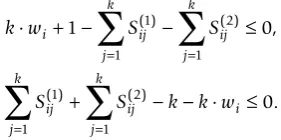
Auxiliary variables and constraints

As mentioned earlier, all variables, including the auxili-ary ones, are Boolean. We take advantage of this, expressing the constraints relating the variables as Boo-lean expressions in terms of the “and’, “or,” “exclusive or,”and“if and only if” operators (denoted by the usual symbols, and, ∧, ∨, , and ⇔, respectively). We then convert these expressions into equivalent linear inequal-ities on zero-one variables using standard techniques [[30], pp. 231-244].

We first describe the variables and constraints that are used to ensure that the settings of the fill-in variables (theFvariables) correspond to a restricted representative

selection. That is, the assignments to the Fvariables

must be such that, for each input treetj, the resulting

plenary splits associated with the tree are pairwise com-patible, so that they yield a plenary treeTj〈tj〉r. For this

purpose, we define variablesCpq, 1 ≤p, q≤mand add

constraints linking these variables and theFvariables such thatCpq= 1 if and only if columnspandqare

com-patible under the fill-in represented by theFvariables. To guarantee that the assignment to theFvariables corre-sponds to a restricted representative selection, we require thatCpq= 1 for every two column indicesp, qthat

corre-spond to splits in the same input tree. We note that the constraints relating the fill-in variablesFand theC -vari-ables closely resemble the ones used by Gusfield et al. [26]. One difference is that for our problem we need“if and only if”relationships, whereas Gusfield et al. require only one direction of the implication.

The constraints on the C-variables use the fact that splitspandqare incompatible if and only if 00, 01, 10,

and 11 all appear in some rows of columnspandq(the

“four gametes condition”). The presence or absence of these patterns for columnspandqis indicated by the set-tings of variables B(_pqab),a, b{0, 1}, where B_pq(ab) = 1 if and only if there is a taxonrsuch thatFrp=aandFrq=b.

The Bpq(ab) are determined from the settings of variables rpq(ab)

, whererranges over the taxa (i.e., the rows ofM (P)). TheΓvariables satisfy (rpqab) ⇔((Frp=a)∧(Frq=b)).

This condition is expressed by the following constraints.

( ) ( ) , ( ) ( ) ( ) (           

1 1 1

1 1 2

a

rp b rq rpqab a

rp b rq rpqa

F F a b

F F   bb a b ) .

  2 (3)

We have that Bpq(ab) ⵪rrpq(ab), which is expressed by

the inequalities below.

    





Observe that Cpq Bpq(00)B(pq01)B(pq10)Bpq(11).

Equivalently we have the constraints below.

B B B B C

B B B

pq pq pq pq pq

pq pq pq

( ) ( ) ( ) ( )

( ) ( )

,

00 01 10 11

00 01

4 4

    

  ((10)_B(11)_{C 4.}

pq pq

(5)

We now consider the variables and constraints that enable us to express the objective function variables. There are three main sets of variables:

•For 1≤ p≤m,Dpequals 1 if and only if columnp

represents the same split as some column with smaller index.

•For 1≤i≤ m, 1≤j≤k, S_ij( )1 , equals 1 if and only if splitiis in treej.

•For 1≤ i≤m, 1≤j≤k, S_ij( )2 equals 1 if and only if splitiis compatible with treej.

As we shall see, the values of thewand thezvariables in the objective function are determined, respectively from the S(1)andS(2)variables, and from thew,S(2), andDvariables.

TheDandS(1)variables depend on variables Epq, 1≤

p, q≤m, where Epq = 1 if and only if columns pand q

of the filled-in matrix represent the same split. Here we have to make a distinction between rooted and unrooted trees. In the rooted case, there exists a root taxonr such thatMri(P) = 1 for every columni. The same is not true

for unrooted trees.

The value ofEpq depends on the patterns that appear

in columns pand q, which can be deduced from the

values of B(_pqab) for different choices of a and b as follows.

• For rooted trees, E_pq  B(_pq01) B_pq(10). This is expressed as follows.

B B E

B B E

pq pq pq

pq pq pq

( ) ( ) ( ) ( ) , . 01 10 01 10 2 2 1   

   (6)

•For unrooted trees, we introduce two auxiliary vari-ables _pq( )1 and _pq( )2 such that

_pq( )1  B_pq(01) B_pq(10) and _pq( )2  B(_pq00) B(_pq11).

Then,

Epq pq( )1 pq( )2.

These logical constraints are expressed by the follow-ing inequalities.

B B

B B

B

pq pq pq

pq pq pq

pq ( ) ( ) ( ) ( ) ( ) ( ) ( ) , ,

01 10 1

01 10 1

00 2 2 1                 B B B E pq pq

pq pq pq

pq pq p

( ) ( ) ( ) ( ) ( ) ( ) , , 11 2

00 11 2

1

2 2

1

   ( )_qq2 _0.

(7)

We are now ready to give the constraints for theD,S(1) andS(2)variables. Observe thatD1= 0 and that, for 1 <p ≤m, Dp ⵪ip11Eip. Equivalently we have

D E

E p D p ip i p ip p i p         





In describing the constraints for theS(1)andS(2) vari-ables, we adopt the convention that the splits of thejth tree correspond to columns j1,..., jd of M(P). Then,

S_ij E_ij E_ij d ( )1

1

  . This translates into the equality

constraint

S_ij E_ij r d r ( ) . 1 1 0   



On the other hand, S_ij( )2 C_ij1 C_ijd. This is equivalent to the two constraints below.

d S C

d S C

ij ij r d ij ij r d r r         





Finally, we describe how the objective function vari-ables relate to the auxiliary varivari-ables. For each i,wi = 1

if and only if Sij k _j Sij

k j

k ( )1 ( )2 1 1   







expressed by the following two constraints.

k w S S

S S k

i ij j k ij j k ij j k ij j k           









1 1 0

1 2 1 1 1 2 1 ( ) ( ) ( ) ( ) ,

 k w_i 0.

(11)

It follows from the definition of the zvariables that, for everyi, j, zij ⇔wi ∧ ¬Sij

( )2 _∧

¬Di. Equivalently we

have the following.

      

   

2 3 0

0

2

2

w S D z

w S D z

i ij i ij

i ij i ij ( )

( )

,

. (12)

there are a total of O(nm2) variables; this number is

dominated by theΓvariables. The total number of

straints for the unrooted case, broken down by con-straint type, is given by the following expression.

4 1 4 1 1 5 1 2

3 4 5

nm m( ) m m( ) m m( ) m m( ) /

( ) ( ) ( ) (

      

        

7 7

8 9 10 11 12

2 1 2 2 2

)

( ) ( ) ( ) ( ) ( )

( )



      

 m mk mk m mkO nm( 2).

The number of constraints for the rooted case is slightly smaller, but of the same order of magnitude. It should be noted that the expressions given in Table 1 assume that all the variables listed are indeed variables. In reality, the values of many of theFvariables are fixed because they correspond to non-question-mark entries inM(P). This in turn fixes the values for severalΓ vari-ables, as well as those of other variables. As a conse-quence, the number of true variables in the ILP formulation is typically much smaller than the worst case estimates in Table 1. In general, the larger the

number of question marks in matrixM(P), the closer

the problem size will be to the worst case estimates. Building Maj+(P)

The ILP model just outlined allows us to find aG〈P〉r

corresponding to some optimal candidate supertree T*.

To build Maj+(P) we need, in principle, the set of all suchG. While there are ways to enumerate this set [31], we have found that an alternative approach works much better in practice. The key observation is that, since Maj +

(P) is the strict consensus of all optimal candidate supertrees, each split in Maj+(P) must also be in T*.

Thus, once we haveT*, we simply need to verify which

splits in T* are in Maj+(P) and which are not. To do this, for each split A|B in T*, we put additional con-straints on the original ILP requiring that the optimal tree achieve an objective value equal or smaller than that ofT* andnot display splitA|B. The resulting ILP has onlyO(mn) more variables and constraints than the original one. If the new ILP is feasible, thenA|B ∉Spl (Maj+(P)); otherwise,A|BSpl(Maj+(P)). We have found that detecting infeasibility is generally much faster than finding an optimal solution.

A data reduction heuristic

The ILP formulation described in the previous section allows us to solve supertree problems of moderate size. Here we describe a data reduction heuristic that allows

us to extend the range of our method significantly in practice, by exploiting the structure that is present in certain supertree problems. Our data reduction heuristic applies when the input profile P = (t1,...,tk) contains a

subset of taxaS that can be treated as a single

super-taxon. Roughly stated, we are looking for a set S such

that every tree in Prespects the split implied byS. We now define this concept more precisely.

Let Spl0(T) denote the set ofallfull splits displayed by T. That is, Spl0(T) includes the non-trivial and the trivial splits displayed byT; in particular,L(T)|∅Spl0(T). We say thatS ⊆L(P) with 1 < |S| < |L(P)| -1 is areducible setif, for each jK, there is a split A|BSpl0(tj) such

that A∩ S=A andB ∩S =∅. Ideally, a reducible set should correspond to a widely-acknowledged biological classification unit. For example, some of the trees in a collection of phylogenies may contain subtrees corre-sponding to different (possibly empty) subsets of the pri-mates. While these subsets may not be identical, and the subtrees may disagree somewhat in their topologies, the input phylogenies are likely to separate primates from non-primates. In settings like this, it makes intuitive sense to restrict our attention to supertrees where redu-cible sets appear as clusters.

Given a reducible setSfor P, we can define two smal-ler subproblems.

•Thereduced profile associated with a reducible set S is the profile PRed (t₁Red,...,t_kRed) where, forkeach j K, tjRed is the tree obtained from tjby contracting the

minimal subtree oftjcontainingS∩L(tj) to a single leaf

nodebS. If S∩L(tj) = ∅, then tjRed =tj. We refer tobS

as thesupertaxon associated with S.

•The satellite profile associated with Sis the profile

PSat (t₁Sat,...,t_kSat) where t_jSat is obtained from tj by

contracting the minimal subtree oftj containing (L(P)

\S)∩ L(tj) to a single leaf node rS. Note that some of

the trees in the satellite profile associated with S may contain onlyrS. Thecompressed satellite profile

asso-ciated with S is the satellite profile associated with S with all of the latter trees removed.

An S-restricted representative selection for P is a selectionR= (T1,...,Tk)〈P〉such that S|(L(P)\S)Spl

(Ti) for all i K. An optimal S-restricted candidate

representative selectionis anS-restricted representative selection Rwith minimum score, and Maj(R) an optimal S-restricted candidate supertree. TheS-restricted major-ity-rule (+) supertree is the strict consensus of all the optimalS-restricted candidate supertrees.

It should be noted that, given an arbitrary reducible

set S, it is not true in general that an optimal S

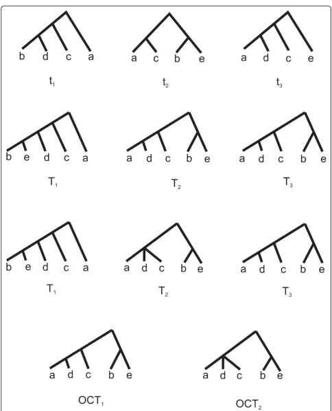
-restricted candidate supertree will be an optimal candi-date supertree, nor that anS-restricted majority-rule (+) supertree will also be a majority-rule (+) supertree. This is illustrated in Figure 1, which shows a profile P= (t1, Table 1 Variables in the ILP formulation

F Γ B δ(i) E C D S(i) w z

mn2m(m-1)n2m(m-1) m(m-1)/2 2m(m-1) 2m(m-1) m mk m mk

The number of variables of each kind is expressed in terms ofn,m, andk, the

t2,t3) where both {b, e} and {b, d} are reducible sets, but where neither optimal candidate tree contains the clus-ter {b, d}, although they both contain {b, e}.

On the other hand, a reducible set may represent use-ful biological knowledge that should be incorporated into a supertree analysis. There are also computational benefits. With the right choice ofS(one where |S| is far

from the extreme values of 2 and |L(P)| -2), the

reduced and satellite profiles can be considerably smal-ler than the original profile, and the corresponding inte-ger programs will have fewer unknown variables. As the following theorem indicates, an optimalS-restricted can-didate supertree can be found by solving the associated subproblems separately and combining their answers.

Theorem 5.Let P be a profile and S be a reducible set in P. Let TRedand TSatbe optimal candidate trees for the reduced profile associated with S and the compressed satellite profile associated with S. Let T be the tree obtained by identifying the nodebS in T

Red

and noderS

in TSat and then suppressing the resulting degree-two vertex. Then, T is an optimal S-restricted candidate supertree for P. Further, if R, is the optimal S-restricted representative selection corresponding to T and RRedand RSatare the optimal representative selections correspond-ing to TRedand TSat, respectively, then s(R) = s(RRed) + s (RSat).

The straightforward proof of this result is omitted. A direct consequence is that the S-restricted majority-rule (+) supertree can be obtained by piecing together the majority-rule (+) supertrees for the reduced and satellite profiles. Observe that if multiple pairwise disjoint redu-cible sets are known, then each of the corresponding compressed satellite profiles can be solved indepen-dently, and the original profile can be reduced by repla-cing each reducible set to a distinct supertaxon. In fact, the idea can be used recursively, so that a satellite pro-file can itself be decomposed to a reduced propro-file and (sub) satellites. As we shall see later, this can result in dramatic problem size reductions.

Results and discussion

Here we report on computational tests with the exact ILP method and the data reduction heuristic. All our experiments were conducted on real data sets, rather than simulated data. We did this because we were inter-ested in seeing if the groupings of taxa generated by majority-rule (+) supertrees would coincide with those commonly accepted by biologists. Another goal of our experiments was to compare the performance of the ILP formulation without data reduction, which we refer to as thebasic method, against that of ILP plus data reduc-tion. All trees considered in our tests were rooted.

To conduct our tests of the basic method, we wrote a program to generate the ILPs from the input profiles.

For our tests of the data reduction heuristic, we used different methods to find reducible sets in a profile; these are outlined later. Given the reducible sets, the corresponding reduced and satellite profiles, as well as the associated ILPs, were generated automatically. All ILPs were then solved using CPLEX (CPLEX is a trade-mark of ILOG, Inc.) on an Intel Core 2 64 bit quad-core processor (2.83 GHz) with 8 GB of main memory and a 12 MB L2 cache per processor.

Experiments with the basic ILP formulation

We tested the basic ILP formulation on five published data sets. The Drosophila Adata set is the example stu-died in [14], which was extracted from a larger Droso-phila data set considered by Cotton and Page [32]. Primates is the smaller of the data sets from [5]. Droso-phila B is a larger subset of the data studied in [32]

than that considered in [14].Chordata A and Bare two

extracts from a data set used in a widely-cited study by Delsuc et al. [33]. Chordata A consists of the first 6 trees with at least 35 taxa (out of 38). Chordata B con-sists of the first 12 trees with at least 37 taxa (out of 38).

The results are summarized in Table 2. Here n, m,

and k are the number of taxa, total number of splits,

and number of trees, respectively.U denotes the

num-ber of question marks inM(P), the matrix representa-tion of the input; Nis the size of the CPLEX-generated reduced ILP. Table 2 shows the time to solve the ILP

and produce an optimal candidate supertree T* and the

time to verify all the splits ofT* to produce Maj+(P).

Experiments with the data reduction heuristic

As a preliminary test, we compared the results obtained via the reduction heuristic with the exact solutions, obtained using the basic ILP method, for two of the data sets listed in Table 2. For simplicity, only clusters from the input trees were used as reducible sets. (Note that unions of input clusters could have also been used as reducible sets.) We wrote a program that chooses clusters greedily. At every step, it selects the largest non-trivial cluster present in some input tree that does not overlap with any of the previously chosen clusters.

an objective value of 8. We found nine pairwise disjoint reducible sets, and built the corresponding reduced and satellite profiles. The reduced profile has an optimal objective value of 8 and all satellite profiles have an optimal objective value of 0.

It should be pointed out that the reducible sets used for Primates and Drosophila B do not necessarily corre-spond to clusters in the majority-rule (+) supertree, although they are displayed by some optimal candidate trees. Thus, one will not obtain a majority-rule (+) supertree by simply composing the solutions to the reduced problems and the satellites. This indicates the importance of choosing relatively few large and well-supported reducible sets. Biological knowledge can serve

as a good guide. For example using the clade

Haplor-rhinias a reducible set for Primates data set, solving the corresponding reduced and satellite profiles and com-bining the respective majority-rule (+) supertrees one gets exactly the same supertree as through the basic (and exact) method. Similarly, using the subgenus Sophophora as a reducible set for Drosophila B, we, obtained precisely the majority-rule (+) supertree for the data set.

Next, we considered some data sets that are well

beyond the reach of our basic ILP method. The

Dro-sphila Cdata set is the full 6-tree Drosophila data set of Cotton and Page [32] from which the Drosophila A and

B data sets were extracted. TheSeabirds data set

con-sists of the 7 trees in the seabirds study by Kennedy and Page [17]; which encompasses 122 taxa (note that one of these taxa is an outgroup, so we do not count it in our study). We also examined the full Chordata set of Delsuc et al. [33], which has 38 taxa and 146 trees. Chordata

We looked for reducible sets in the full Chordata data set by considering increasingly larger subprofiles, start-ing with one input tree and then includstart-ing one more input tree at every step. For each subprofile, we con-ducted an exhaustive search for reducible sets. The number of reducible sets increased at first, then fluctu-ated, and finally declined. After the 20th tree, there were no reducible sets. Thus, the data reduction heuris-tic proved to be ineffective for this data set.

Drosophila C

We identified seven reducible sets for Drosophila C. Six of these were found by the greedy approach; the seventh

corresponded to the subgenus Sophophora (the latter

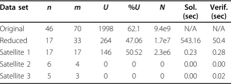
was selected manually, after some of the subproblems identified by our program proved impossible to solve). Four of the associated satellites were trivially solvable, since each contained only two taxa. We then solved ILPs for the reduced and the nontrivial satellites. The running time statistics are summarized in Table 3, which shows the same kind of data shown in Table 2, except that this time it reports these statistics for the original, reduced and satellite problems. Notably, even though the original ILP was too large to be solved, the reduced profile was solved in less than 10 minutes and the satellite profiles were solved almost instantly.

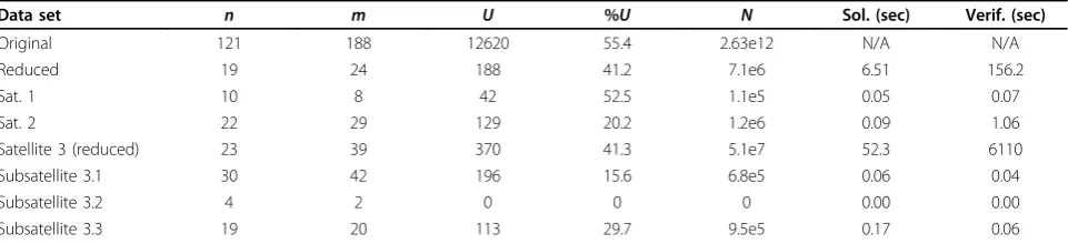
Seabirds

To handle the Seabirds data set, we identified three reducible sets, which yielded a reduced profile and three satellite profiles, numbered 1, 2, and 3. Satellite profile 3 was too big to be solved by the basic ILP method, so it was further reduced by identifying three reducible sets within it, which resulted in three (sub-) satellite profiles, numbered 3.1, 3.2, and 3.3. The various reducible sets correspond to biologically meaningful classification units, as we explain next. In what follows, we refer to Table 2 Summary of experimental results with the basic ILP method

Data set n m k U %U N Sol. (sec) Verif. (sec)

Drosophila A 9 17 5 60 39.2 9.8 e5 0.83 1.6

Primates 33 48 3 590 37.3 7.8 e7 15.83 2.86

Drosophila B 40 55 4 1133 51.5 1.25 e9 362 19

Chordata A 38 290 6 330 3 1.40 e8 120 258

Chordata B 38 411 12 306 2 1.05 e8 986 1784

Size and solution times for the ILP formulations of the various data sets. HereUdenotes the number of question marks inM(P), the matrix representation of the

input;Nis the size of the CPLEX-generated reduced ILP;n,m, andkare as in Table 1. Shown are the time to solve the ILP and produce an optimal candidate

supertreeT* and the time to verify all the splits ofT* to produce Maj+

(P).

Table 3 Results of Drosophila C analysis using data reduction

Data set n m U %U N Sol. (sec)

Verif. (sec)

Original 46 70 1998 62.1 9.4e9 N/A N/A

Reduced 17 33 264 47.06 1.7e7 543.16 50.4

Satellite 1 17 17 146 50.52 2.3e6 0.23 0.28

Satellite 2 6 4 0 0 0 0.00 0.00

Satellite 3 5 3 0 0 0 0.00 0.02

Size and solution times for all six trees in trees in Cotton and Page’s

the 7 input trees of Kennedy and Page’s seabirds data set by the same letters A-G that those authors used in [17].

Satellite 1 comprises the familySpheniscidae

(Pen-guins, 10 taxa), which agrees with widely-accepted clas-sifications for seabirds [34]. Members of this family appear in input trees E, F, and G of [17], and clearly form clusters of their own. Satellites 2 and 3 correspond toDiomedeinae (Albatrosses, 22 taxa), and Procellarii-nae(gadfly petrels, shearwaters, fulmars and diving pet-rels, 73 taxa). This agrees with the Sibley-Ahlquist classification [35] (represented by tree G). The resulting reduced profile has 19 taxa (16 original taxa and three supertaxa).

Satellite 3 (Procellariinae) has three subsatellites. Satellite profile 3.1 comprises the genusPterodroma(30 taxa). Satellite 3.2 is for genusPelecanoides (four taxa). Satellite 3.2 is a combination ofPuffinusand Calonectris (10 taxa), which is supported by [36] (tree E). With

these three sub-satellites, the reduced Procellariinae

profile has 23 taxa (20 original taxa and three supertaxa).

Table 4 summarizes the results on the Seabirds data set. The majority-rule (+) supertree is shown in Figure 2, along with the MRP strict consensus tree of [32]. While the original problem was too big for CPLEX to solve on our machine, the reduced model was solved in 6.5 seconds. Most subproblems were solved and verified in a negligible amount of time. A notable exception was the reduced version of satellite 3, which required almost a minute to solve and nearly one hour and 45 minutes to verify.

Discussion

Our results using the basic ILP formulation compare well with the published ones. For Drosophila A we obtained exactly the same tree reported in [14]. For Pri-mates, the output is exactly the same as [5], which was produced by PhySIC method. The coincidence with PhySIC is noteworthy, since this supertree is less

controversial than the MRP, Mincut, and PhySICPC supertrees reported in [5]. The reason for the coinci-dence may lie in the fact that, while heuristic, PhySIC requires that all topological information contained in the supertree be present in an input tree or collectively implied by the input trees, which bears some similarity

with properties (CW1)-(CW4) of majority (+)

supertrees.

For Drosphila B, Cotton and Page [32] show four supertrees: strict consensus of gene tree parsimony (GTP), Adams consensus of GTP, strict consensus of MRP, Adams consensus of MRP. Among the 10 clusters found by our ILP, two are in all four of these supertrees, three are found in the Adams consensus of GTP and Adams consensus of MRP, one is in the strict and Adams consensus of GTP, and one is found in the strict and Adams consensus of MRP. Thus, with only four input trees we were able to generate a tree that is quite similar to the published results. For Chordata A, the 12 splits found matched published results [33] exactly. For Chordata B, the 14 splits found matched [33].

We have not mapped out the precise boundary within which it is feasible to use the basic ILP method. How-ever, it appears that it may not extend much beyond the dimensions of the problems listed in Table 2. For exam-ple, Drosophila B contains four out of 6 of the trees stu-died in [32]. Adding a fifth tree to the data set yields a problem that could not be solved by the basic ILP method. A major factor here is that the size of our ILP grows as the square of the total number of splits in all trees, and the solution time is exponential in the worst case. Incorporating a new tree to Drosophila B could easily add enough splits to the problem to put it well beyond the reach of our technique. We should add that model size does not appear to be the sole factor that

makes instances hard— sparsity also seems to play a

role. Drosophila C

The majority-rule (+) supertree for Drosphila C con-structed by our method (available upon request) has 15

Table 4 Results of Seabirds analysis using data reduction

Data set n m U %U N Sol. (sec) Verif. (sec)

Original 121 188 12620 55.4 2.63e12 N/A N/A

Reduced 19 24 188 41.2 7.1e6 6.51 156.2

Sat. 1 10 8 42 52.5 1.1e5 0.05 0.07

Sat. 2 22 29 129 20.2 1.2e6 0.09 1.06

Satellite 3 (reduced) 23 39 370 41.3 5.1e7 52.3 6110

Subsatellite 3.1 30 42 196 15.6 6.8e5 0.06 0.04

Subsatellite 3.2 4 2 0 0 0 0.00 0.00

Subsatellite 3.3 19 20 113 29.7 9.5e5 0.17 0.06

nontrivial clusters, while the MRP strict consensus tree of Cotton and Page [32] has 11. Of these only three appear in both trees. This rather surprising result moti-vated us to try to assess how well the input trees are represented by the supertree. To this end, we relied on the notions of support and conflict, along the lines pro-posed by Wilkinson et al. [37].

Let tbe an input tree for a profileP,Tbe a supertree forP, andS be a non-trivial cluster inT (i.e.,Sdoes not contain the root ofT andS|(L(P)\S)Spl(T)). Let S’= S∩ L(t). We say that treet supports SifS’is a non-tri-vial cluster int. Tree tisin conflict with SifS’is incom-patible with t; i.e., there is no tree t’with L(t’) = L(t) such that Spl(t)∪ {S’|(L(t)\S’)} ⊆ Spl0(t’). If t neither supports nor is in conflict withS, we say that tis irrele-vanttoS.

Theorem 1 hints that each cluster S in the

majority-rule (+) supertree should have more input trees support-ing it than contradictsupport-ing it, even when most trees are irrelevant toS. This indeed holds for the Drosophila C majority-rule (+) supertree: Every one of its non-trivial clusters is supported by at least one input tree and does not conflict with any input tree. In contrast, of the five clusters in the MRP strict consensus supertree for which support outweighs conflict, only three have no conflict with any input tree. Of the remaining clusters, three have the same amount of conflict as support, and for three others the amount of support is outweighed by the amount of conflict. In fact, among the latter, there is a cluster that is in conflict with five out of six of the input trees; the remaining tree is irrelevant to that clus-ter. We refrain from claiming the superiority of one supertree over the other, since the biological relevance of both trees needs to be studied in more detail.

Seabirds

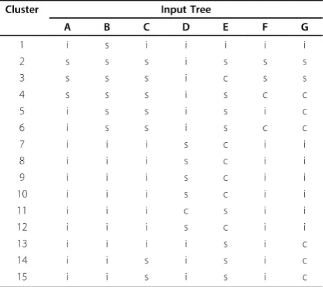
Figure 2 compares the majority-rule (+) supertree for the seabirds data set, constructed using the data reduc-tion heuristic, with the MRP strict consensus supertree that Kennedy and Page presented for the same data set [17]. The latter is the strict consensus of 10,000 equally parsimonious trees obtained using MRP. There are 66 nontrivial clusters in the majority-rule (+) supertree, compared with 75 nontrivial clusters in the MRP strict consensus tree (ignoring the outgroup). Among these clusters, 63 are present in both trees (95% of 66 and 84% of 75). The reducible sets used to construct the majority-rule (+) supertree are indicated by heavy lines. Note that these sets are also clusters in the MRP supertree.

Three clusters, numbered 1-3 in Figure 2, are in the majority-rule (+) supertree but not in the MRP tree; 12 clusters, numbered 4-15 in Figure 2, appear in the MRP tree but not in the majority-rule (+) tree. For each of the seven input trees (labeled A-G in [17]) and each of

these 15 clusters, Table 5 indicates whether the tree supports, is in conflict with, or is irrelevant to the clus-ter. As Theorem 1 would lead us to expect, each of clusters 1-3 (from the majority-rule (+) tree) has more input trees supporting it than in conflict with it. Of the 12 clusters (4-15) that are present only in the MRP strict consensus tree, seven have as many trees in sup-port as in conflict. The others have more supsup-port than conflict.

In general, it appears that MRP may have a bias toward preserving clusters that are present in trees that contain many members of the families represented in those clusters. This is noticeable for Pterodroma, where the disagreement between trees D and E is resolved in favor of the former five times to one, in clusters 7, 8, 9, 10, and 12 versus cluster 11. This may be related to the

“size bias” that previous researchers have observed in MRP [38]: Here, even though E is the larger tree (90

taxa versus 30), D has more taxa in the Pterodroma

genus (30 versus 16). Majority-rule (+) trees seem not to have such a bias, because the expansion process used to construct representative selections tends to put all input trees, regardless of their size, on equal footing. These are, of course, only preliminary observations; this issue clearly deserves further analysis.

Conclusions

Our results indicate that the majority-rule (+) method produces biologically reasonable phylogenies (i.e., phylo-genies with no unsupported groups), and that the Table 5 Support and conflict for the Seabirds data set

Cluster Input Tree

A B C D E F G

1 i s i i i i i

2 s s s i s s s

3 s s s i c s s

4 s s s i s c c

5 i s s i s i c

6 i s s i s c c

7 i i i s c i i

8 i i i s c i i

9 i i i s c i i

10 i i i s c i i

11 i i i c s i i

12 i i i s c i i

13 i i i i s i c

14 i i s i s i c

15 i i s i s i c

method is practical for medium-scale problems. Unfor-tunately, while polynomial, the size of our ILP is quad-ratic in the total number of splits in the input trees. This, together with the fact that solving the ILP takes exponential time in the worst case limits the range of applicability of the basic ILP formulation. It also explains in part why the addition of a single tree to a data set can convert a tractable problem into an intract-able one. More extensive tests are needed to assess the limitations of the basic ILP approach accurately. In any event, our computational experience shows that the technique does handle some real, biologically significant, problems nicely. Moreover, our results suggest that the ILP approach, in combination with our data reduction heuristic is a promising way to tackle larger problems.

Acknowledgements

The authors benefited greatly from discussions with James Cotton, William HE Day, RC Powers, and Mark Wilkinson. We thank Frédéric Delsuc for providing us the data set from [33]. This work was supported in part by the National Science Foundation under grants DEB-0334832 and DEB-0829674.

Author details

1_{Department of Computer Science, Iowa State University, Ames, IA 50011,} USA.2Department of Applied Mathematics, Illinois Institute of Technology, Chicago, IL 60616, USA.

Authors’contributions

JD developed the methods, programmed them, conducted the

computational experiments, and wrote the first draft of the manuscript. DFB supervised the work of JD, and contributed to the method development, the experimental design, and to the writing of the manuscript. FRMcM contributed to the theoretical foundations of the method, especially to the formulation and proof of Theorem 1; he also contributed to the writing of the manuscript.

Competing interests

The authors declare that they have no competing interests.

Received: 11 August 2009

Accepted: 4 January 2010 Published: 4 January 2010

References

1. Gordon AD:Consensus supertrees: The synthesis of rooted trees containing overlapping sets of labelled leaves.Journal of Classification

1986,9:335-348.

2. Bininda-Emonds ORP, Cardillo M, Jones KE, MacPhee RDE, Beck RMD, Grenyer R, Price SA, Vos RA, Gittleman JL, Purvis A:The delayed rise of present-day mammals.Nature2007,446:507-512.

3. Bininda-Emonds ORP, Ed:Phylogenetic Supertrees: Combining Information to Reveal the Tree of Life, Volume 4 of Series on Computational BiologyBerlin: Springer 2004.

4. Wilkinson M, Cotton JA, Lapointe FJ, Pisani D:Properties of supertree methods in the consensus setting.Systematic Biology2007,56:330-337. 5. Ranwez V, Berry V, Criscuolo A, Fabre PH, Guillemot S, Scornavacca C,

Douzery EJP:PhySIC: A veto supertree method with desirable properties. Systematic Biology2007,56(5):798-817.

6. Adams EN:Consensus techniques and the comparison of taxonomic trees.Systematic Zoology1972,21(4):390-397.

7. Bryant D:A classification of consensus methods for phylogenetics. Bioconsensus, Volume 61 of Discrete Mathematics and Theoretical Computer ScienceProvidence, RI: American Mathematical SocietyJanowitz M, Lapointe FJ, McMorris F, B Mirkin B, Roberts F 2003, 163-185.

8. Day W, McMorris F:Axiomatic Consensus Theory in Group Choice and BiomathematicsPhiladelphia, PA: SIAM Frontiers in Mathematics 2003.

9. Barthélemy JP, McMorris FR:The median procedure for n-trees.Journal of Classification1986,3:329-334.

10. Margush T, McMorris FR:Consensus n-trees.Bulletin of Mathematical Biology1981,43:239-244.

11. Amenta N, Clarke F, St John K:A linear-time majority tree algorithm.Proc. 3rd Workshop Algs. in Bioinformatics (WABI_’03), Volume 2812 of Lecture Notes in Computer ScienceSpringer-Verlag 2003, 216-226.

12. Pattengale ND, Gottlieb EJ, Moret BME:Efficiently computing the Robinson-Foulds metric.Journal of Computational Biology2007,14(6):724-735. 13. Robinson DF, Foulds LR:Comparison of phylogenetic trees.Mathematical

Biosciences1981,53:131-147.

14. Cotton JA, Wilkinson M:Majority-rule supertrees.Systematic Biology2007,

56:445-452.

15. Goloboff PA, Pol D:Semi-strict supertrees.Cladistics2005,18(5):514-525. 16. Dong J, Fernández-Baca D:Properties of majority-rule supertrees.

Systematic Biology2009,58(3):360-367.

17. Kennedy M, Page RDM:Seabird supertrees: combining partial estimates of procellariiform phylogeny.The Auk2002,119(1):88-108.

18. Baum BR:Combining trees as a way of combining data sets for phylogenetic inference, and the desirability of combining gene trees. Taxon1992,41:3-10.

19. Ragan MA:Phylogenetic inference based on matrix representation of trees.Molecular Phylogenetics and Evolution1992,1:53-58.

20. Swofford D:PAUP*: Phylogenetic analysis using parsimony (*and other methods).Sinauer Assoc., Sunderland, Massachusetts, U.S.A. Version 4.0 beta. 21. Goloboff P:Minority rule supertrees? MRP, compatibility, and minimum

flip may display the least frequent groups.Cladistics2005,21:282-294. 22. Pisani D, Wilkinson M:MRP, taxonomic congruence and total evidence.

Systematic Biology2002,51:151-155.

23. Brown DG, Harrower IM:Integer programming approaches to haplotype inference by pure parsimony.IEEE/ACM Trans Comput Biol Bioinformatics

2006,3(2):141-154.

24. Gusfield D:Haplotype inference by pure parsimony.CPM, Volume 2676 of Lecture Notes in Computer ScienceSpringerBaeza-Yates RA, Chávez E, Crochemore M 2003, 144-155.

25. Gusfield D:The multi-state perfect phylogeny problem with missing and removable data: Solutions via integer-programming and chordal graph theory.RECOMB, Volume 5541 of Lecture Notes in Computer Science

SpringerBatzoglou S 2009, 236-252.

26. Gusfield D, Frid Y, Brown D:Integer programming formulations and computations solving phylogenetic and population genetic problems with missing or genotypic data.COCOON, Volume 4598 of Lecture Notes in Computer ScienceSpringerLin G 2007, 51-64.

27. Sridhar S, Lam F, Blelloch GE, Ravi R, Schwartz R:Mixed integer linear programming for maximum-parsimony phylogeny inference.IEEE/ACM Trans Comput Biol Bioinformatics2008,5(3):323-331.

28. Semple C, Steel M:PhylogeneticsOxford Lecture Series in Mathematics, Oxford: Oxford University Press 2003.

29. Steel MA:The complexity of reconstructing trees from qualitative characters and subtrees.Journal of Classification1992,9:91-116. 30. Sierksma G:Linear and Integer Programming, Theory and PracticeNew York,

NY: Marcel Dekker 1996.

31. Danna E, Fenelon M, Gu Z, Wunderling R:Generating multiple solutions for mixed integer programming problems.Integer Programming and Combinatorial Optimization, Volume 4513 of LNCSBerlin: Springer-VerlagFischetti M, Williamson DP 2007, 280-294.

32. Cotton JA, Page RDM:Tangled trees from molecular markers: reconciling conflict between phylogenies to build molecular supertrees.Phylogenetic Supertrees: Combining Information to Reveal the Tree of Life, Volume 4 of Series on Computational BiologyBerlin: SpringerBininda-Emonds ORP 2004, 107-125. 33. Delsuc F, Brinkmann H, Chourrout D, Philippe H:Tunicates and not

cephalochordates are the closest living relatives of vertebrates.Nature

2006,439:965-968.

34. Brooke MdL:Seabird systematics and distribution: a review of current knowledge.Biology of Marine BirdsBoca Raton, Florida: CRC pressSchreiber EA, Burger J 2002, 57-85.

35. Sibley CG, Ahlquist JE:Phylogeny and Classification of Birds: A Study in Molecular EvolutionNew Haven, Connecticut: Yale University Press 1990. 36. Nunn GB, Stanley SE:Body size effects and rates of cytochrome b

evolution in tube-nosed seabirds.Molecular Biology and Evolution1998,

37. Wilkinson M, Pisani D, Cotton JA, Corfe I:Measuring support and finding unsupported relationships in supertrees.Systematic Biology2005,

54(5):823-831.

38. Purvis A:A modification to Baum and Ragan_’s method for combining phylogenetic trees.Systematic Biology1995,44:251-255.

doi:10.1186/1748-7188-5-2

Cite this article as:Donget al.:Constructing majority-rule supertrees. Algorithms for Molecular Biology20105:2.

Submit your next manuscript to BioMed Central and take full advantage of:

• Convenient online submission

• Thorough peer review

• No space constraints or color figure charges

• Immediate publication on acceptance

• Inclusion in PubMed, CAS, Scopus and Google Scholar

• Research which is freely available for redistribution