Bayesian Approach in Estimation of Scale Parameter of Nakagami Distribution

(1)

Scale Parameter of Nakagami Distribution

Azam Zaka

Punjab Education Department Lahore, Pakistan

Ahmad Saeed Akhter

College of Statistical & Actuarial Sciences University of the Punjab, Lahore, Pakistan [email protected]

Abstract

Nakagami distribution is a flexible lifetime distribution that may offer a good fit to some failure data sets. It has applications in attenuation of wireless signals traversing multiple paths, deriving unit hydrographs in hydrology, medical imaging studies etc. In this research, we obtain Bayesian estimators of the scale parameter of Nakagami distribution. For the posterior distribution of this parameter, we consider Uniform prior, Inverse Exponential prior and Levy prior. The three loss functions taken up are Squared Error Loss Function (SELF), Quadratic Loss Function (QLF) and Precautionary Loss Function (PLF). The performance of an estimator is assessed on the basis of its relative posterior risk. Monte Carlo Simulations are used to compare the performance of the estimators. It is discovered that the PLF produces the least posterior risk when uniform priors is used. SELF is the best when inverse exponential and Levy Priors are used.

Keywords: Nakagami distribution, bayesian estimation, square error loss function, quadratic loss function, precautionary loss function.

1. Introduction

Nakagami distribution was proposed for modeling the fading of radio signals (Nakagami, 1960). Numerous parametric models are used in the analysis of lifetime data and in problems related to the modeling of failure processes. Among univariate models, a few particular distributions occupy a central role because of their demonstrated usefulness in a wide range of situations. This category contains the Exponential, Weibull, Gamma and Lognormal distributions.

(2)

In physics, if you observe a gas at a fixed temperature and pressure in a uniform gravitational field, the height of the various molecules also follow an approximate Nakagami distribution. Nakagami distribution is also used in lifetime distribution model i.e. the analysis of failure times of electrical components. On the other hand the Nakagami distribution is the best distribution to check the reliability of electrical component as compare to the Weibull, Gamma and lognormal distribution.

The probability density function of the distribution is given as

2 ₂ ₁

(x, , ) ₂

( )

f _x _e

x

 _

  _ _

 

  

 ; x > 0 (1)

Where, 0is the shape parameter and  0 is scale parameter, also

mean=

1/ 2 ( 1/ 2) 

 

   

 

  and variance =

1/ 2

1 ( 1/ 2)

1

( )

 

 

 __{ } _ 

 _ 

  _  

 

 

 

. It collapses to

Rayleigh distribution when = 1 and half normal distribution= 0.5

(3)

the scatterer concentration based on data obtained using a non-focused transducer. Schwartz et al. (2011) developed and evaluated analytic and bootstrap bias-corrected maximum likelihood estimators for the shape parameter in the Nakagami distribution. It was found that both “corrective” and “preventive” analytic approaches to eliminating the bias are equally, and extremely, effective and simple to implement. Dey (2012) obtained Bayes estimators for the unknown parameter of inverse Rayleigh distribution using Squared error and Linex loss function. Kazmi et al. (2012) compared class of life time distributions for Bayesian analysis. They studied properties of Bayes estimators of the parameter using different loss functions via simulated and real life data. Feroze (2012) discussed the Bayesian analysis of the scale parameter of inverse Gaussian distribution. Feroze and Aslam (2012) found the Bayesian estimators of the scale parameter of Error function distribution. Different informative and non-informative priors were used to derive the corresponding posterior distribution. Ali et al. (2012) discussed the scale parameter estimation of the Laplace model using different asymmetric loss functions. Yahgmaei (2013) proposed classical and Bayesian approaches for estimating the scale parameter in the inverse Weibull distribution when shape parameter is known. The Bayes estimators for the scale parameter is derived in Inverse Weibull distribution, by considering Quasi, Gamma and uniform priors under square error, entropy and precautionary loss function. Zaka and Akhter (2013) derived the different estimation methods for the parameters of Power function distribution. Zaka and Akhter (2013) discussed the different modifications of the parameter estimation methods and proved that the modified estimators appear better than the traditional maximum likelihood, moments and percentile estimators.

2. Posterior Distributions under the Assumption of Different Priors

The objective of this chapter is to find Bayesian estimators of the scale parameter of Nakagami distribution under various loss functions and priors. A comparison of these estimates is also made.

An obvious choice for the non-informative prior is the Uniform distribution. The Uniform Prior relating to the scale parameter  is defined as:

P( ) k

The likelihood function of Nakagami distribution is

 





2 ₂ ₁

( | ) exp

2

( ) 0

1 n

n

L x x_i n

n n _i _X

i i



 _ _



 _

 

 

 

  



   



 

  _ _



 

( | ) exp

2

1 n

L x n

X i i  

 



 

 

  



 _ _



 

 _ 

(4)

The Posterior distribution of scale parameter  using uniform prior is

0

( ) ( | ) ( | )

( ) ( | )

P L x

P x

P L x d

       



Therefore exp 2 1 ( | ) exp 2 0 1 n n X i i P x n _d n X i i        _           _ _     _          _ _ _ _        _    1 2 _exp ( ) 2 1 1 ( | ) (n 1) n n n X n i _X i _i i P x                      _   _ _    

  ; 1/n (2)

Now we use Inverse Exponential Prior and Levy Prior as informative prior because they are compatible with the parameter  of the Nakagami distribution. Similarly Posterior distributions using informative priors for the parameter  of the Nakagami distribution are derived below:

Inverse Exponential Prior relating to the scale parameter  is:

1 1

( ) exp

2

P  _

 

    

 _ _ 0  

Then the Posterior distribution of scale parameter  using Inverse Exponential Prior is

0

( ) ( | ) ( | )

( ) ( | )

P L x

P x

P L x d

       



1

1 ₂ 1 ₂ 1

( ) ( ) 2exp 1 1 ( | ) (n 1) n n n X X n i i i i P x      _ _ _    _      _  _      

(5)

Now the Levy Prior relating to the scale parameter  is given as:

3 / 2

( ) _{exp 2}

2

d d

P  _ _

  

 

 _ _ 0  

Similarly the Posterior distribution of scale parameter  using Levy Prior is

0

( ) ( | ) ( | )

( ) ( | )

P L x

P x

P L x d

       



1/ 2 1

2 3 / 2 2

( ) exp ( )

2 2

1 1

( | )

(n 1/ 2)

n

n _d n _d

n X X i i i i P x          _ _       _  _     

  (4)

3. Bayesian Estimation Under Three Loss Functions

In statistics and decision theory a loss function is a function that maps an event into a real number intuitively representing some "cost" associated with the event. Typically it is used for parameter estimation, and the event in question is some function of the difference between estimated and true values for an instance of data. The use of above lemma is made for the derivation of results.

3.1. Squared Error Loss Function (SELF)

The squared error loss function proposed by Legendre (1805) and Gauss (1810) is defined as:



 



2

,

L  _SELF  _SELF

The derivation of Bayes estimator under SELF using Uniform Prior is given below:

E( | )x

SELF 

 

0

E( | ) x  P( | )x d  



0 1 2 _exp ( ) 2 1 1 E( | )

(n 1) n n n X n i _X i _i i x d                         _   _ _      







2 1 E( | )

2 n X i i x SELF _n        

 ; 2 /n (5)

3.2. Quadratic Loss Function (QLF)

A quadratic loss function is defined as:

  



2

x c t x

(6)

For some constant C, the value of the constant makes no difference to a decision, and can be ignored by setting it equal to 1.

The quadratic loss function can also be defined as



,



QLF 2

L _QLF          _ _  

The Bayes estimator under QLF using Uniform Prior is 1

E( | ) 2 E( | )

x QLF x       0 1 1

E( | )x  P( | ) x d 

 _

_



1

2 _exp

( ) ₂

1

1 1

E( | )

(n 1) 0 n n n X n i _X i _i i x d                        _   _ _  _ _ _  _{ }   



1



1 E( | )

2 1 n x n X i i      _  

; 1/n

Now

0

2 2

E( | )x  P( | ) x d   _

_

 1 2 _exp ( ) 2 1 1 2 2

E( | )

(n 1) 0 n n n X n i _X i _i i x d   _                     _   _ _  _ _ _  _{ }   



1



2 E( | )

2 2 1 n n x n X i i      _       _   

; 1/n

(7)

3.3. Precautionary Loss Function (PLF)

Norstrom (1996) introduced an asymmetric precautionary loss function (PLF) which can be presented as:



,

 

PLF



2

L  _PLF  



 

Similarly the Bayes estimator under PLF using Uniform Prior is derived as:





1/ 2

2 E( | )x PLF   





1 2 _exp ( ) 2 1 1 1

2 2 2

E( | )

(n 1) 0 n n n X n i _X i _i i x d                        _   _ _  _ _ _

  _ _ ; 1/n





1

_

_

2

_

1

2 2

E( | )

2 3 n X i i x PLF n n         

  ;  3 /n (7)

4. Posterior Risks Under Different Loss Functions

The Posterior risk of the Bayes estimator under different Loss functions using Uniform Prior are:

Using Square Error Loss function (SELF):





2

( ) E( | ) E( | )

P _SELF   x   x



 



2 2 1 ( ) 2 2 3 n X i i P _SELF n n           _    

  ; 3 /n (8)

Quadratic Loss function (QLF):





2

1 E( | )

( ) 1

2 E( | )

x P _QLF x       _ 1 ( ) P _QLF n    (9)

Precautionary Loss Function (PLF):





( ) 2 E( | )

(8)





 



2 2

1 1

( ) 2

2

2 3

n n

X X

i i

P _PLF

n

n n

 





 

 

 

 

 _ _ 

 _  _



 

 

 

;  3 /n (10)

Similarly the expressions for Bayes Estimators and Risks under Inverse Exponential and Levy Priors can be derived in a similar manner.

5. Simulation Study

Using Easy fit Software, we have generated 5,000 Random numbers from Nakagami Distribution with different values of Parameters  and. A program has been developed in R language to obtain the Bayesian Estimates and Posterior Risks under 10,000 replications and averages of 10,000 outputs has been presented in the tables below.

Table 1: Bayes Estimates under (= 1.5,  = 2)

Sample Size

Uniform Prior

= 1.5,  = 2

Inverse Exponential Prior Levy Prior

n SELF QLF PLF SELF QLF PLF SELF QLF PLF 5 2.69602 1.97708 2.98057 2.10068 1.65843 2.25649 2.18454 1.69908 2.35957 20 2.10873 1.96815 2.14742 2.00535 1.88002 2.03964 2.01842 1.89027 2.05352 40 2.03689 1.96900 2.05468 1.98259 1.91864 1.99932 1.99478 1.92991 2.01175 100 1.99738 1.97075 2.00416 1.98018 1.95413 1.98682 1.97990 1.95376 1.98655 150 1.98925 1.97157 1.99373 1.97504 1.95763 1.97944 1.97767 1.96020 1.98209 250 1.98216 1.97158 1.98482 1.97469 1.96421 1.97733 1.97712 1.96662 1.97976 400 1.97873 1.97213 1.98038 1.97238 1.96583 1.97403 1.97449 1.96793 1.97614

Table 2: Bayes Estimates under (= 1,  = 0.5)

Sample Size

Uniform Prior

= 1,  = 0.5

(9)

Table 3: Bayes Estimates under (= 1,  = 2)

Sample Size

Uniform Prior

= 1,  = 2

Table 4: Bayes Estimates under (= 2,  = 1.5)

Sample Size

Uniform Prior

= 2,  = 1.5

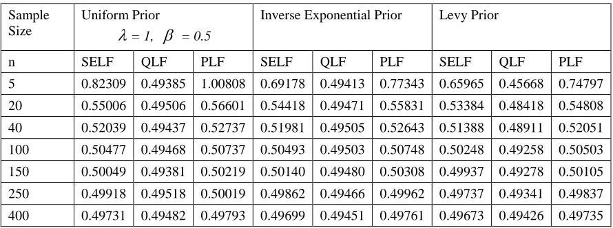
Table 5: Posterior Risks under (= 1,  = 0.5)

Sample Size

Uniform Prior

= 1,  = 0.5(p)

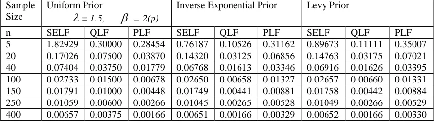
Table 6: Posterior Risks under (= 1.5,  = 2)

Sample Size

Uniform Prior

= 1.5,  = 2(p)

(10)

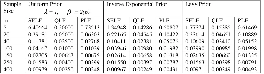
Table 7: Posterior Risks under (= 1,  = 2)

Sample Size

Uniform Prior

= 1,  = 2(p)

Table 8: Posterior Risks under (= 2,  = 1.5)

Sample Size

Uniform Prior

= 2,  = 1.5(p)

6. Summary and Conclusions

The posterior risk based on all priors and for all loss functions, relating to the scale parameter of a Nakagami distribution, expectedly decrease with the increase in sample size. Using the Uniform prior, the posterior risk increases with increase in the value of β whatever the value of λ may be. At the same level of β, the posterior risk decreases with for a Nakagami distribution with a larger λ. For the same unknown β value, the posterior risk decreases for a Nakagami distribution with a larger λ. The performance of loss function is dependent on the values of λ and β jointly. Using all Priors, the posterior risk is inversely proportional to the choice of values of the β.

The posterior risk using Uniform prior is independent of the parameter β, but it tends to increase for larger values of the parameter λ of Nakagami distribution. The posterior risk after checking the effect of hyper parameter using Inverse Exponential and Levy Priors is also free of β, but for the fixed λ, the posterior risk decreases with increase in β.

(11)

When λ= 1.5 and λ =2 and all values of β for n=5 and for n=20 and above for all values of λ, β the PLF under Uniform prior shows minimum posterior risk than Levy prior and Inverse Exponential prior. Affect of hyper Parameters did not affect the mentioned results. The PLF of Uniform prior showed Least Posterior risk than Levy and Inverse Exponential Priors. While in all other cases of SELF and QLF informative Priors give better results than uninformative Uniform prior.

References

1. Aalo, V. A. (1995). Performance of maximal-ratio diversity systems in a correlated Nakagami fading environment. IEEE Transactions on Communication, 43(8), 2360-2369.

2. Abid, A. and Kaveh, M. (2000). Performance comparison of three different estimators for the Nakagami m parameter using Monte Carlo simulation. IEEE Communications Letters, 4, 119- 121.

3. Ali, S., Aslam, M., Kazmi, S.M.A. and Abbas, N. (2012), Scale Parameter Estimation of the Laplace Model Using Different Asymmetric Loss Functions, International Journal of Statistics and Probability, 1 (1), 105-127.

4. Cheng, J. and Beaulieu, N. C. (2001). Maximum likelihood estimation of the Nakagami m parameter. IEEE Communications Letters, 5(3), 123-132.

5. Dey, S. (2012). Bayesian estimation of the parameter and reliability function of an inverse Rayleigh distribution. Malaysian Journal of Mathematical Sciences, 6(1), 113-124.

6. Feroze, N. and Aslam, M. (2012). A note on Bayesian analysis of error function distribution under different loss functions. International Journal of Probability and Statistics, 1(5), 153-159.

7. Feroze, N. (2012). Estimation of scale parameter of inverse gausian distribution under a Bayesian framework using different loss functions. Scientific Journal of Review, 1(3), 39-52.

8. Hoffman, C. W. (1960). The m-Distribution, a general formula of intensity of rapid fading. Statistical Methods in Radio Wave Propagation: Proceedings of a Symposium held June 18-20, 1958, 3-36. Pergamon Press. 2.

9. Kazmi, A. M. S, Aslam, M. and Ali, S. (2012). Prefernece of prior for the class of life-time distributions under different loss functions. Pak.J.Statist, 28(4), 467-487. 10. Kim, K. and H. A. Latchman (2009). Statistical traffic modeling of MPEG frames size experiments and analysis. Statistical Methods in Radio Wave Propagation, 29(3), 456-465.

11. Smolikova, R., Wachowiak, P. M. and Zurada, M. J. (2004). An information-theoretic approach to estimating ultrasound backscatter characteristics. Computers in Biology and Medicine, 34, 355-270.

12. Sarkar, S., Goel, N. and Mathur, B. (2009). Adequacy of Nakagami-m distribution function to derive GIUH. Journal of Hydrologic Engineering, 14(10), 1070-1079.

(12)

14. Schwartz, J. Gowdin, T. R. and Giles, E. D. (2011). Improved maximum likelihood estimation of the shape parameter in the Nakagami distribution. Mathematics Subjects Classification, 62, 30-36.

15. Srivastava, U. (2012). Bayesian estimation of shift point in Poisson model under asymmetric loss function. Pak.J.Stat.Oper.Res, 8(1), 31-42.

16. Tsui, P., Huang, C. and Wang, S. (2006). Use of Nakagami distribution and logistic compression in ultrasonic tissue characterization. Journal of Medical and Biological Engineering, 26(2), 69-73.

17. Tsui, H., Chang, C., Ho, M. C., Lee, Y., Chen, Y., Chang, C., Huang, N. and Chang, K. (2009). Use of Nakagami statistics and empirical mode decomposition for ultrasound tissue characterization by a nonfocused transducer. Ultrasound in Medicine & Biology, 35(12), 2055-2068.

18. Batah, F. M., Ramanathan, T. V. and Gore, S. D. (2008). The Efficiency of Modified Jackknife and Ridge type regression estimators. A comparison. Surveys in Mathematics and its Applications, 3, 111-122.

19. Singh. (1986). An almost unbiased ridge estimator. The Indian Journal of Statistics, 48(B), 342-346.

20. Vinod, H. D. and Ullah, M. (1981). Recent Advances in Regression Methods. New York M. Dekker.

21. Wackerly, D. D., Mendenhall, W. and Scheaffer, R. L. (2008). Mathematical Statistics with Applications, 7, Thomson.

22. Wimmer, G. and Witkovsky, V. (2002). Proper rounding of the measurements results under the assumption of Uniform distribution. Measurement Science Review, 2, 1-7.

23. Yang, D. T. and Lin, J. Y. (2000). Food Availability, Entitlement and the Chinese Femine of 1959-61. Economic Journal, 110, 136-58.

24. Yahgmaei, F. Babanezhad, M. and Moghadam, S.O. (2013). Bayesian estimation of the scale parameter of inverse Weibull distribution under the asymmetric loss functions. Journal of Probability and Statistics.

25. Zaka, A. and Akhter, A. S. (2013). Methods for estimating the parameters of the Power Function Distribution. Pakistan Journal of Statistics and Operational Research, 9(2), 213-224.

26. Zaka, A. and Akhter, A. S. (2013). A note on Modified Estimators for the Parameters of the Power Function Distribution. International Journal of Advanced Science and Technology, 59, 71-84.