https://doi.org/10.5194/os-14-525-2018
© Author(s) 2018. This work is distributed under the Creative Commons Attribution 4.0 License.
Assimilating high-resolution sea surface temperature data improves
the ocean forecast potential in the Baltic Sea
Ye Liu1and Weiwei Fu2
1Swedish Meteorological and Hydrological Institute, Norrköping 60176, Sweden
2Department of Earth System Science, University of California Irvine, Irvine, CA 92697, USA Correspondence:Ye Liu ([email protected])
Received: 25 January 2018 – Discussion started: 13 February 2018 Revised: 8 June 2018 – Accepted: 11 June 2018 – Published: 25 June 2018
Abstract. We assess the impact of assimilating the satellite sea surface temperature (SST) data on the Baltic forecast, particularly on the forecast of ocean variables related to SST. For this purpose, a multivariable data assimilation (DA) sys-tem has been developed based on a Nordic version of the Nu-cleus for European Modelling of the Ocean (NEMO-Nordic). We use Kalman-type filtering to assimilate the observations in the coastal regions. Further, a low-rank approximation of the stationary background error covariance metrics is used at the analysis steps. High-resolution SST from the Ocean and Sea Ice Satellite Application Facility (OSISAF) is assimi-lated to verify the performance of the DA system. The as-similation run shows very stable improvements of the model simulation as compared with both independent and depen-dent observations. The SST prediction of NEMO-Nordic is significantly enhanced by the DA forecast. Temperatures are also closer to observations in the DA forecast than the model results in the water above 100 m in the Baltic Sea. In the deeper layers, salinity is also slightly improved. In addition, we find that sea level anomaly (SLA) is improved with the SST assimilation. Comparisons with independent tide gauge data show that the overall root mean square error (RMSE) is reduced by 1.8 % and the overall correlation coefficient is slightly increased. Moreover, the sea-ice concentration fore-cast is improved considerably in the Baltic Proper, the Gulf of Finland and the Bothnian Sea during the sea-ice formation period, respectively.
1 Introduction
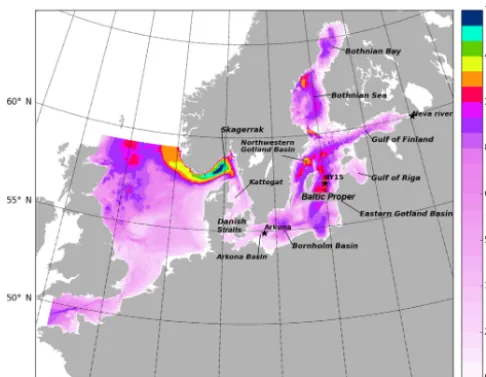
Monitoring the marine status of the Baltic Sea with relevant resolution and accuracy is a key requirement to serve the ma-rine policy for detecting the influence of human activities on the environment and better understanding the response of ocean to accelerating global climate change. The Baltic Sea is one of the largest brackish seas in the world. It is a semi-enclosed basin, whose hydrography is highly variable and in-fluenced by large-scale atmospheric processes and significant influx of freshwater from river runoff and precipitation (Lep-päranta and Myrberg, 2009). In addition, the water exchange between the North Sea and Baltic Sea through the Danish Straits is hindered by shallow topographic restrictions in the transition zone (Fig. 1).
Me-Figure 1.Geographical domain and bathymetry (in meters) of the NEMO-Nordic configuration.
teorological and Hydrological Institute’s (SMHI) needs to is-sue well-informed forecasts and warnings for decision mak-ing by other authorities durmak-ing, e.g., severe weather events, but also to the public. To improve the forecast quality, the core three-dimensional dynamic model of the SMHI oper-ational forecast system has recently migrated to the Nordic version of the Nucleus for European Modelling of the Ocean (NEMO-Nordic).
In additional to model development, an extended observa-tional network has been established by the joint efforts of the countries surrounding the Baltic Sea. The observation plat-forms include vessels, buoys, coastal stations, satellites, etc. Specially, the observations from satellites have dominated the coverage of sea surface temperature (SST) observational networks in the Baltic Sea (She et al., 2007). Among satel-lite products, the SST is most popularly and widely used for the operational forecast, reanalysis or validation of the model because of both its coverage and properties. SST acts as a medium between atmospheric and oceanic variations through activation of coupling mechanisms. SST is also a key ocean variable to link many processes that occur in the upper ocean, for example, air–sea exchange of energy, primary productiv-ity and formation of water masses.
A realistic forecast of SST is essential to an ocean fore-casting system. SST is especially important for the Baltic Sea because the average water depth is only 56 m and its surface water is directly related to the bottom water by the mixing in the shallow sub-basins. Recently, the applications of SST for forecasting and analyzing the status of the North Sea and Baltic Sea have received particular attention. In the short-term forecast, Losa et al. (2012, 2014) investigated the systematic model uncertainties for forecasting in the North Sea and Baltic Sea by assimilating the Advanced Very High Resolution Radiometer (AVHRR) SST data. Nowicki et
al. (2015) applied SST observed from the Moderate Resolu-tion Imaging Spectroradiometer (MODIS) aboard the Aqua satellite into 3-D coupled ecosystem model of the Baltic Sea with the Cressman analysis scheme. O’Dea et al. (2012) en-hanced the SST prediction skill of the operational system by assimilating both in situ data and level 2 SST data pro-vided by the Global Ocean Data Assimilation Experiment High-Resolution SST (GHRSST) into a European northwest shelf operational model. Moreover, SST has been used in the long-term analysis in this region. For instance, Stramska and Bialogrodzka (2015) analyzed spatial and temporal variabil-ity of SST in the Baltic Sea based on 32 years of satellite data, which indicate that there is a statistically significant trend of increasing SST in the entire Baltic Sea. However, these long-term SST data have not been used to verify the application of sophisticated data assimilation (DA) methods for hydrog-raphy model in the Baltic profiles’ simulation, especially at the Baltic deep water regions. Another important question is what amount of satellite SST can improve long-term forecast of ocean variables related to SST in the Baltic Sea.
The objective of this study is to address the impact of as-similating a high-resolution SST product on the forecast of the Baltic Sea, particularly the forecast of SST-related vari-ables like sea level and sea ice. It is also the first time that satellite SST from the Ocean and Sea Ice Satellite Applica-tion Facility (OSISAF) was assimilated into NEMO-Nordic model (NEMO variant for the North Sea and Baltic Sea). For operational forecast, the SST from OSISAF is the most important dataset in the Baltic Sea because it differs from hindcast-analyzed products like OSTIA (Operational SST and Sea Ice Analysis) data. As a level 2 product, the OS-ISAF SST has both good temporal and spatial coverage in the Baltic Sea. As there is no hindcast information included in the OSISAF SST, we are able to assess direct impacts of assimilating SST observations. Therefore, exploring the po-tential of this product is critically important to further im-proving the new operational forecast system. In addition, our study will enrich the reanalysis database of the Baltic Sea. In this study, we use the local singular evolutive interpo-lated Kalman (LSEIK) filter (Pham, 2001) to account for the model uncertainties arising from a wide range of spatial and temporal scales (Haines, 2010). One of our focuses is the im-pact of assimilating SST on the modeled sea level and the sea ice in the Baltic Sea. For the whole Baltic Sea, how the SST assimilation influences the temperature and salinity (T/S) at different depths is another focus of this study.
2 Methodology 2.1 NEMO-Nordic
NEMO-Nordic has been set up at SMHI for the North Sea and the Baltic Sea (Hordoir et al., 2015) (Fig. 1). Open boundaries are implemented in the northern North Sea tween Scotland and Norway, and in the English Channel be-tween Brittany and Cornwall, respectively (Hordoir et al., 2013). In this study, NEMO-Nordic employs a horizontal res-olution of 2 nautical miles (3.7 km) and 56 vertical levels, and with a vertical resolution of 3 m close to the surface, decreas-ing to 22 m at the bottom of the deepest part of the Norwe-gian trench. NEMO-Nordic uses a fully nonlinear, explicit free surface (Adcroft and Campin, 2004). A bulk formula-tion is used for the surface boundary condiformula-tion (Large and Yeager, 2004). The ocean model is coupled to the Louvain-la-Neuve (LIM3) sea-ice model (Vancoppenolle et al., 2008) with a constant value of 10−3psu for the sea-ice salinity. A time-splitting approach is used to compute a barotropic and a baroclinic mode, as well as the interaction between them. A tidal inversion model is used to define the barotropic mode at the open boundary conditions (Egbert and Erofeeva, 2002). A total of 11 tidal harmonics are defined for sea level and barotropic tidal velocities. In addition, a coarse-resolution barotropic storm surge model covering a large area of the northern Atlantic Basin provides wind-driven sea level that is added to the tidal contribution. TheT/S data at the open boundary are provided by the Levitus climatology (Levitus and Boyer, 1994). Radiation conditions are applied to cal-culate baroclinic velocities at these boundaries. A quadratic friction is applied with a constant bottom roughness of 3 cm, and the drag coefficient is computed for each bottom grid cell. NEMO-Nordic uses a total variation diminishing (TVD) advection scheme with a modified leapfrog approach that en-sures a very high degree of tracer conservation (Leclair and Madec, 2009). Unresolved vertical turbulence is parameter-ized with κ−ε scheme (Umlauf and Burchard, 2003). In addition, Galperin parameterization is used to obtain a sta-ble long-term stratification for the Baltic Sea (Galperin et al., 1988).
A Laplacian isopycnal diffusion is used for both momen-tum and tracers with a diffusion parameter that is constant in time but varies in space. Additional strong isopycnal dif-fusion is used close to the Neva River inflow (Gulf of St. Petersburg) in order to avoid negative salinities. The bottom boundary layer is parameterized to ease the propagation of saltwater inflows between the Danish Straits and the deepest layers of the Baltic Sea (Beckmann and Döscher, 1997). A free-slip option is used for lateral boundaries.
The model is forced by meteorological forcing derived from a downscaled run of Euro4M reanalysis (Dahlgren et al., 2014). The downscaling is based on the regional atmo-spheric model RCA4 (Samuelsson et al., 2011) which uses the reanalysis data as boundary conditions. A runoff database provides the river flow to NEMO-Nordic (Donnelly et al., 2016); it includes interannual variability for the Baltic Sea basin and is based on climatological values for the North Sea basin. The salinity of the river runoff is set to a constant value of 10−3psu, which is the same value used for the sea ice to avoid any negative salinity.
2.2 Local singular evolutive interpolated Kalman (LSEIK) filter
The method used to assimilate SST into NEMO-Nordic is the local singular evolutive interpolated Kalman (LSEIK) fil-ter (Pham, 2001; Nerger et al., 2006). This is a sequential data assimilation scheme, which is an error subspace ex-tended Kalman filter that uses a minimum number of ensem-ble members to reduce the prohibitive computation burden (Pham, 2001). The LSEIK filter produces the correction for the model state by weighting the difference between the ob-servations and the model state estimation. The weight coef-ficients are constructed by the model error covariance ma-trix and observation error covariance mama-trix. Similar to other ensemble-based data assimilation methods, the LSEIK filter uses the spread of the sample ensemble to estimate the un-certainties of the model state. Further, a forgetting factorρ
is introduced to parameterize the imperfect model by am-plifying the already existing modes of the background error (Pham et al., 1998; Pham, 2001). Furthermore, the LSEIK filter is based on an explicit low-rank approximation of the model error covariance matrix. A second-order exact sam-pling method is used to initialize the LSEIK filter (Pham, 2001). Localization was also used to remove the unrealistic long-range correlation with a quasi-Gaussian function and a uniform horizontal correlation scale (Liu et al., 2013). It was performed by neglecting observations that were beyond cor-relation distance from an analyzed grid point. In other words, only data located in the “neighborhood” of an analyzed grid point should contribute to the analysis at this point (Liu et al., 2009; Janji´c et al., 2011).
3 Observations
3.1 Satellite observations
(the EUMETSAT MetOp-A and NOAA-18, -19) with the AVHRR instrument. The SST product has a resolution of 5 km and is produced twice daily at 00:00 and 12:00 UTC. It covers the Atlantic Ocean from 50 to 90◦N. The SST observations are thermal infrared observations from the AVHRR instrument and are therefore limited by cloud cover (Kilpatrick et al., 2001). The cloud mask in use is based on a multispectral thresholding algorithm by SMHI. The products were retrieved using a nonlinear split win-dow algorithm (Walton et al., 1998). The coefficients in the retrieval algorithm are determined through regression toward in situ observations, and the dataset thus represents the sub-skin temperature of the oceans. Further, sub-skin observations are subject to diurnal warming effects, which can be significant in the Baltic Sea. Here, only the sub-skin SST at night (00:00 UTC), which is comparable to in situ (buoy) measurement, is used to minimize this effect. The SST is controlled with the climatology check. A quality level from 0 to 5 is associated with every pixel. The higher the level value, the better the quality of the observations (Brisson et al., 2002). Observations with quality level 4 (good) or 5 (excellent) are collected for the analysis, and low-quality observations were removed. By applying the above quality control processes, only a subset of the original OSISAF products is kept in this study. Based on the former validation, a bias value of 0.5◦C is given for this product.
Further, the IceMap from a sea-ice concentration dataset with a high spatial resolution of 5 km (https://www.smhi.se/ klimatdata/oceanografi/havsis, 8 February 2018) is used to validate the DA results. It is produced by SMHI and origi-nates from digitized ice charts. An advantage of these data is that the ice charts are quality checked manually. However, the drawback is that they include some subjective steps. The temporal resolution of the IceMap SST is twice a week in the experimental period. Sea ice occurs most frequently in the Bay of Bothnia, with up to 100 ice-covered days per year. However, sea ice can occur in all parts of the Baltic Sea and Danish Straits, demonstrating the need for careful treatment of sea ice in the SST analysis.
3.2 In situ data
The observations from the German Maritime and Hy-drographic Agency (BSH) moored buoy stations were collected as an independent dataset to validate the as-similation results. The observations have high tempo-ral resolution and a long continuous record. The second dataset was downloaded from the Swedish Oceanographic Data Centre SHARK database (http://sharkweb.smhi.se, 8 February 2018). SHARK mainly contains low-resolution conductivity–temperature–depth (CTD) data from a list of predefined standard stations in the Baltic Sea, as well as in Kattegat and Skagerrak. Only observations that have passed gross quality control procedures are collected into the SHARK database. This procedure includes, for example,
location checks and local stability checks. In addition, vali-dated data records from tide gauges are also used. The sea level anomaly measurements from tide gauges (sea level sta-tions) are measured in a local height system, and values are presented relative to theoretical mean sea level, a level cal-culated from many years of annual means, which takes into account the effect of land uplift and sea level rise. The values are averaged over a 1 h period.
Not all the available observations from satellites, moored buoys, CTDs and tide gauges were included in this study. To obtain the high assimilation quality results, another quality control was applied for these data before they were used in assimilation and validation. These controls include examina-tion of forecast observaexamina-tion differences by excluding those observations for which the difference between the forecast and the measurement exceeded given standard maximum de-viations. The criteria were set up empirically based on past validation results of the model (Liu et al., 2013). Further-more, stations located on land, according to the NEMO-Nordic grid, were excluded. We also removed the duplicate records of these data.
The accuracy of observation error is difficult to be defined for all water points. The observation is commonly assumed to be spatially irrelevant, which results in an error covari-ance matrix that is time-invariant diagonal and its diagonal elements equal the variance of observation error. The error for an observation used in data assimilation mainly includes the representation error and the measurement error. The mea-surement error arises primarily from the meamea-surement device alone, the temporary reading error and imperfect retrieval al-gorithm. According to Janji´c et al. (2017), the representa-tion error in data assimilarepresenta-tion comprises the error due to un-solved scales or processes, the preprocessing error and the observation-operator error. In this study, the observation er-ror was estimated to one value as the sum of all observa-tion uncertainties used in the analysis. In addiobserva-tion, the un-certainties of satellite SST vary from the coast to the open sea, i.e., higher uncertainties in the coastal region relative to the open sea. We used a constant standard deviation value of 0.4◦C based on the standard deviation of satellite SST, which ranged from the∼0.1 to∼0.5◦C in the Baltic Sea (She et al., 2007; Høyer et al., 2016).
4 Configuration of LSEIK in the experiment
183 state vectors, which includes sea level, temperature and salinity, in total to describe the model variability because suc-cessive states are quite similar. The initial ensemble provided an estimate of the initial model state and its uncertainty be-fore the assimilation of SST observations. The quantity of the model variability was expected to be reasonably compa-rable with the forecast error, which was dominated by mis-placement of mesoscale features and varied in location and intensity seasonally. Further, the very high frequencies of model variability were also unfavorable in an ensemble of state vectors for SST data assimilation (Oke et al., 2005). Therefore, a band-pass filter was used to remove the un-wanted frequency of model variability. To initial the low-rank error covariance matrix, a multivariable empirical orthogonal function (EOF) analysis was applied on the 183 state vec-tors of model variables (sea level, temperature and salinity). In the North Sea and Baltic Sea, error covariances of dif-ferent variables are not uniform and strongly dependent on whether the variable resides in the open sea or coastal zone. Each state variable was then normalized by the inverse of its spatially averaged variance at every model level. At last, 34 leading EOF modes were kept and they explained 85 % over-all variability. Then, the initial error covariance matrix was estimated byPa(t0)≈L0U0LT0, where theL0is composited by the leading EOF modes andU0is diagonal matrix with the corresponding eigenvalues on its diagonal. We used a time-invariant sample ensemble to approximate the background error covariance during the experimental period (Korres et al., 2012; Liu et al., 2017). This stationary ensemble affords a good approximation of the ocean’s background error co-variance. Meanwhile, it is computationally efficient for our objective.
The localization scale is another import factor to the as-similation system, especially at the coastal region. Large cor-relation scale may transfer artificial increments to the po-sitions far away from the analysis observation during the DA process. However, the small correlation scale is prone to cause the singularity of ocean state around analyzed observa-tion and break the continuity of the ocean state. Hence, an un-reasonable scale causes the instability of the model integra-tion or degrades the assimilaintegra-tion quality. Unfortunately, the accuracy length for the correlation is unknown for the North Sea and Baltic Sea. The correlation length scale is to some extent dependent on the Rossby radius of deformation (Losa et al., 2012), which varies from∼200 km in the barotropic mode to∼10 km or even less in the baroclinic mode (Fennel et al., 1991; Alenius et al., 2003). According to the former research like Liu et al. (2013, 2017), a length scale of 70 km was specified for both the North Sea and Baltic Sea in this study. Note that this value may be not perfect and more ac-curate correlation length needs to be tested for LSEIK. For example, spatially variable length scales are the next step for the regional DA simulations.
To define the forgetting factor, a 1-month simulation ex-periment with varying the factorρwas done in January 2010.
At last, a factorρ=0.3 resulted in the best assimilation per-formance. Further, we define a 2-day assimilation window in assimilation experiment. As a result, the observations in the 2 days before the assimilation time were used to calculate the innovation with observation operator. When we calculated the innovation, we also changed the observation error accord-ing to the observation time byε=0.4×exp(−0.151t ); here,
1tis the absolute time difference between observation time and DA time.
5 Results
In the following subsections, we conducted two runs with and without assimilation of the SST observations from the OSISAF database, both runs with the above setup of the anal-ysis system. Accordingly, the runs with and without assim-ilation are called ASSIM and FREE, respectively. We con-sidered the evolution of SST based on 48-hourly local anal-ysis from 1 January to 31 December 2010. The 48-hourly forecast SST from two runs was assessed with observations from different datasets. Then, we analyzed the impact of the data assimilation on the profile simulation ofT/S. At last, we evaluated the system performance with respect to sea surface anomaly and sea ice, respectively.
5.1 Comparison with satellite data
First, we presented two cases to show the ocean state before and after the assimilation of the OSISAF SST data in Fig. 2. The first case was given at 11 January 2010, a date with clear weather and many observations available. The model has ob-vious difficulties in reproducing the observed SST. The cold biases in the forecast were found in the Skagerrak, west coast of the Baltic Proper and the Bothnian Bay, respectively. How-ever, the warm biases appeared in the interior of the Baltic Sea and the Kattegat. The largest deviation in FREE reached 2.2◦C at the Skagerrak. Apparently, temperature by assimila-tion analysis agreed with the satellite-derived data much bet-ter. This correction at the analysis step has allowed us to re-duce the deviation of the SST forecast from the observations. The DA system simulation was also verified on 2 June 2010, which has also many available OSISAF observations. The bi-ases on 2 June 2010 were obviously different from those on 11 January 2010. Moreover, it was found they had a roughly opposite bias signal. For example, relative to the OSISAF SST at the Baltic Proper, Bothnian Sea and Bothnian Bay, FREE produced relatively warmer water on 11 January and colder water on 2 June (Fig. 2), respectively. After data as-similation, the analysis increments were appropriately added to the model field. In general, the SST DA has improved the simulated SST in both cases (Fig. 2).
AS-Figure 2.Map of SST from FREE(a, e), OSISAF(b, f), ASSIM(c, g)and the assimilation increments(d, h)on 11 January 2010(a–d)and 2 June 2010(e–h), respectively.
SIM had different distributions in the Baltic Sea. In general, FREE had smaller error in the Skagerrak, the eastern Katte-gat and the interior of the Bothnian Sea relative to other sub-basin of the Baltic Sea. The largest RMSE was found at the connection region between the Baltic Proper and the Both-nian Sea. This could be caused by the shallow water, com-plicated bathymetry and large observation biases in this area. It was also noted that the RMSE was larger in the coastal region compared to its interior in the Baltic Proper and Both-nian Sea. After the assimilation, the SST was significantly improved. The RMSE of SST from ASSIM was generally smaller than 1.0◦C. However, there were still some regions where the improvements were relatively small and the RMSE of SST was greater than 1.0◦C. These large errors were pre-dominantly located at the edge of the Baltic Sea and the Dan-ish Straits. For instance, the RMSE of SST was greater than 1.2◦C at both the entrance of the Gulf of Finland and the west coast of the Bothnian Sea. The relatively small improve-ments were regularly caused by the rare observations or the less accurate observations near the coastal water.
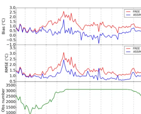
The overall daily averaged SST errors against the IceMap observations have been estimated (Fig. 4). The observations had better coverage in summer and autumn than in winter and spring. The variability of the number of observations directly affected the assessment of DA results. The model biases had pronounced seasonal variability, which had small values in spring and winter. In general, the assimilation provided bet-ter SST estimations. The free run had a RMSE of 1.47◦C. After the assimilation, the RMSE was reduced to 1.03◦C, whereas the bias was reduced by 0.73◦C. An interesting fea-ture was that the SST error reduction due to the assimilation was almost consistent with the variability of the number of
IceMap observations. For example, the improvement became larger with the increasing number of IceMap observations from March to June 2010. However, the number of obser-vations was kept constant during the period June–November 2010 and the improvement shown in both the bias and RMSE of SST did not exhibit large variability, which meant reliable performance of the DA system.
5.2 Comparison with independent in situ data
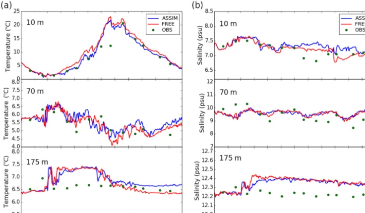
The time series ofT/Swere compared with independent ob-servations located at the Arkona station (54.88◦N, 13.87◦E) in the Arkona Basin and at BY15 (57.33◦N, 20.05◦E) in the Eastern Gotland Basin, respectively. These two stations were selected to verify the experiment results because of their rel-atively completed observation records for the experimental period. In the Arkona Basin, the water depth was shallow and the water column can be well mixed between the surface and bottom water. Thus, the bottomT/Swas largely affected by the surface dynamic (Liu et al., 2014). Relative to obser-vations, the model had warm biases at this station (Fig. 5). At a depth of 25 m, the observed temperature showed the largest variability, which was a good representation of the bottom characteristics of the mixed layer. In mid-August, the temper-ature was abruptly increased by 10◦C at a depth of 25 m and
sta-Figure 3.Map of the RMSE of SST from ASSIM(a)and FREE(b)calculated against IceMap SST in 2010, respectively.
Figure 4.The evolution of basin-averaged bias and RMSE of SST from FREE and ASSIM relative to IceMap SST and the number of IceMap observations in 2010.
tion, the surface observations were missing; the comparison at 7 m depth verified the subsurface simulations. The ob-servations showed larger salinity variability in winter rela-tive to summer. This pronounced seasonal variation is asso-ciated with the variation of fresh river runoff and netE–P
(evaporation–precipitation) flux (Fu et al., 2012). At a depth of 7 m, salinity was obviously underestimated from April to September and overestimated after November, although ASSIM had slightly better results compared to FREE. The DA also provided better simulation of salinity at 25 m depth. For example, the salinity bias in the October was reduced by 3 psu by DA. At a depth of 40 m, the saltwater inflows were observed, resulting in sudden increases of salinity. For
instance, the salinity was increased by 3.5 psu in February followed by a decreasing trend. The variations were repro-duced in both FREE and ASSIM, whereas the intensity of the decreased process is weakly simulated with a difference of 3 psu, and the inflow in March was not strong enough rel-ative to the observed one. Observations also showed that a large salinity variability amounts to 4–8 psu in the autumn. Although FREE and ASSIM had shown these changes, their magnitude was obviously weaker than observations. The pos-sible reason was that the model’s resolution was inadequate to well resolve the topography and eddies in this area. Both the large runoff and the complicated bathymetry posed chal-lenges for the model to tackle the small-scale dynamic pro-cess in such a shallow basin. A higher-resolution model per-haps was more preferable to study this dynamic process.
Figure 5.The time series of temperature(a)at depths of 0, 25 and 40 m and salinity(b)at depths of 7, 25 and 40 m at the Arkona station (54.88◦N, 13.87◦E), respectively.
FREE. This result might be explained by the fact that the strong correlation is not expected between surface and lay-ers below the halocline because of the strong stratification in this basin, which perhaps yield the artificial correction. Therefore, the improvement of the surface temperature can-not guarantee its positive influence on the bottom tempera-ture. To the salinity, the model had less accurate simulation with generally low salinity biases at 10 m depth. ASSIM pro-vided better salinity simulation compared to FREE. At 70 m depth, the small variation of salinity was found after DA. Moreover, at 175 m depth, the observation had very small variability (about 0.1 psu). In general, both experiments have reproduced these variations. However, FREE increased salin-ity by 0.2 psu from March to April relative to the observa-tion, which caused the overall salinity overestimated amount to 0.2 psu. This increasing process was not shown in obser-vations and the reason remained unclear. The DA has shown slight improvement, but it is still saltier than the observations. The mixed layer depth (MLD) was calculated at the Arkona and BY15 stations and compared with the SHARK observations in Fig. 7. We used the temperature criterion to define the MLD, i.e., the depth at which the temperature de-viated from the surface value by 0.5◦C (Fu et al., 2012). Fig-ure 7 shows that the MLD at the Arkona station had larger variability relative to the MLD at BY15. The reason for this feature is that the deeper water at Arkona is easily affected by wind forcing because of the shallow bathymetry and well mixing, whereas the temperature variation in the upper wa-ter at BY15 has difficulty influencing the deeper wawa-ter be-cause of the strong stratification. Both runs had reproduced the MLD variability feature similarly to the observations. For example, the minimum MLD appeared in summer, which
was about several meters. The assimilation of satellite SST caused strong changes in the MLD at both stations, espe-cially in winter. One explanation was that the Baltic Sea was largely affected by wind forcing and the winter wind was much stronger than the summer wind. Further, strong heating in summer promoted stratification in summer and shoaled the MLD.
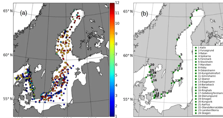
Further, the temporal and spatial distribution of the SHARK observations is shown in Fig. 8a. These observations were unevenly distributed in the Baltic Sea. In the Skager-rak, the observations appeared at the Danish and Swedish coast. However, in the Bornholm Basin, Kattegat and Baltic Proper, the observations mainly were found in the central and the Swedish coast sides. There were also many obser-vations in the Bothnian Sea and rare obserobser-vations in the cen-tral part of the Bothnian Bay. It must be noticed that there are no SHARK observations in both the Gulf of Finland and Gulf of Riga during the experimental period. Moreover, these SHARK profiles in the first 4 months were mainly located in the Skagerrak to the Baltic Proper, which are relatively rare in the northern Baltic Sea. In the Bothnian Bay, the observa-tions are mainly in the winter period.
Figure 9 shows the change of overall bias and RMSE of
Figure 6. The time series of temperature(a)and salinity (b)at the BY15 station (57.33◦N, 20.05◦E) at depths of 10, 70 and 175 m, respectively.
Figure 7.The time series of mixed layer depth at the Arkona and BY15 stations.
the RMSE in ASSIM was reduced by 5.59 and −20.31 % above and below 100 m relative to FREE, respectively. Below 90 m, the temperature was also overadjusted, which changed the warm bias to cold bias. It is worth noting that the num-ber of the deeper water observations in the transition zone is substantially less than that in the Baltic Sea. For the salinity, both RMSE and bias of ASSIM showed very minor changes relative to FREE inside the Baltic Sea. For the water above 100 m, the total RMSE of salinity was increased by 3.48 % (from 1.15 psu in FREE to 1.19 psu in ASSIM) in the
transi-tion zone and 1.04 % (from 0.96 psu in FREE to 0.97 psu in ASSIM) in the Baltic Sea.
5.3 Sea level anomaly
SLA represents a vertically integrated effect of theT/S vari-ations over the whole water column. The accurate simulation of SLA is thus a good indicator of the model performance. Therefore, validating the impact of SST assimilation on the simulation of SLA is very important to the Baltic Sea fore-cast. The observations from the 24 tide gauge stations were used. These gauge stations are mainly located on the Swedish coast (see Fig. 8b). Since only the SST is assimilated in this study, the SLA observations are completely independent.
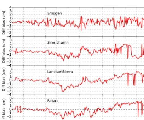
We calculated the RMSE and correlation coefficients for both FREE and ASSIM against the observations from tide gauges (Fig. 10). The overall RMSE was reduced by 1.8 % and the correlation coefficients were slightly increased. Among these stations, RMSE at Oskarshamn was decreased by 5.6 %, which is larger than that at other stations. The min-imum RMSE change of SLA was seen at Klagshamn. For the correlation coefficient, improvement in the SLA by the DA is very small. The Simrishamn station showed the biggest change of correlation coefficient, which is 1.1 %. The RMSE and correlation comparison demonstrated that the SST DA has generally positive effects on the forecast of the SLA.
Figure 8. (a)Map of the temperature and salinity profiles from the SHARK database in 2010. The colors show the observation months.
(b)The tide gauge stations along the Swedish coast.
Figure 9. The overall RMSE and bias of temperature(a, b)and salinity(c, d)from FREE and ASSIM relative to observations as a function of water depth inside(b, d)and outside(a, c)of the Baltic Sea.
variability of the SLA difference between two experiments at the Smogen station had higher frequency compared to other stations. The reason was that the Smogen station was located at the transition zone where the water had higher frequency variations caused by the brackish Baltic in-/outflowing water relative to other three stations. At these four stations, the im-provements were mainly in late spring and summer, whilst the degraded simulations were mostly after mid-September, respectively. The SST assimilation had less impact in late winter and early spring compared to other seasons. In ad-dition, the impact of SST assimilation on SLA simulation was not the same at the four positions. For instance, dur-ing the period from mid-November to mid-December, the SLA in ASSIM was improved at Simrishamn and degraded at both the Ratan and Landsort Norra stations, respectively. This phenomenon was possibly caused by the imperfect cor-relation between SST and SLA in the stationary samples. Further, these steric small changes of SLA by DA were what we expected because only SST was assimilated into NEMO-Nordic.
5.4 Sea ice
Figure 10.The improvement (%) of correlation and RMSE for the SLA at the tide gauge stations. The station positions are shown in Fig. 8b.
Figure 11.The variation of SLA biases in ASSIM relative to FREE against observations as a function of time. The station positions are shown in Fig. 8b.
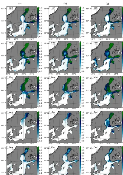
in Figs. 12–13. In contrast to the daily evaluation in Losa et al. (2014), the monthly mean SIC was used to represent the general status of sea ice in the Baltic Sea. In addition, SIC in January, February and December showed the variation of the sea ice in winter.
In January 2010, the observations showed large ice cover-age in the Bothnian Bay and the Gulf of Finland, and small SIC in the Gulf of Riga, respectively. Models generally re-produced this distribution of sea ice. However, FREE simu-lated too much sea ice in the Gulf of Finland and the east-ern coast of the Baltic Proper relative to the observations.
closer to that in IceMap in Bothnian Sea. In the Gulf of Fin-land and Gulf of Riga, the SIC error was increased in ASSIM. In April, the large SIC error in FREE was shown in the Both-nian Sea, BothBoth-nian Bay, Gulf of Riga and Gulf of Finland, where no clear improvements were seen in ASSIM. In De-cember, sea-ice coverage was smaller because of relatively warm temperature compared to that in other winter months. Most of the sea ice with high concentration was observed at the edge of the Bothnian Bay. Nevertheless, high concentra-tion ice in FREE also formed at the transiconcentra-tion zone between the Bothnian Sea and Bothnian Bay. Relatively, ASSIM re-duced the high concentration biases of sea ice. By contrast, both ASSIM and FREE had lower concentration ice than ob-servations on the eastern coast of the Bothnian Sea. The SIC from ASSIM was relatively lower than that from FREE in the northern Finish coast, whereas the observations had high concentration ice there.
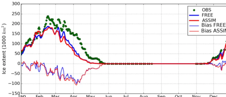
The daily SIE from FREE and ASSIM was compared with observations in Fig. 13. The observed SIE was generally in-creased from January to February and reached the maximum in mid-February. During the period of March–May, SIE was decreased as temperature was increasing. SIEs in both FREE and ASSIM experiments were generally underestimated by comparison with the observations in 2010, especially in the period from mid-March to early April. The SIE bias in both runs was roughly increased from January to early April. In early April, the maximum negative bias of SIE was found to be 105 000 km2 for ASSIM and 10 000 km2for FREE. The impact of SST assimilation on the SIE was positive during the phase of sea-ice formation. For example, the SIE bias was reduced by 25 000 km2 at the end of February and in mid-December. However, during the phase of sea-ice melting (March to April), the SIE error was increased in ASSIM even with the decreased error of SST. For example, the SIE bias in ASSIM was increased by 42 000 km2relative to FREE in the early March. These increased SIE error in March mainly happened in the Gulf of Riga and Gulf of Finland.
6 Conclusion and discussions
A DA system based on a LSEIK filter has been coupled to the NEMO circulation model of the North Sea and Baltic Sea. The method was successfully applied for assimilating high-resolution satellite SST data. We demonstrated that, over the period of 2010, the agreement of the SST forecast with the in-dependent satellite observation was improved by∼29.93 % in comparison with the regular forecast without DA. The as-similation quality is directly related to the number of obser-vations.
Compared with independent in situ data from SHARK, the RMSE of temperature was reduced by 21.38 and 5.59 % for the water above 100 m inside and outside of the Baltic Sea, respectively. However, in the deeper layers, the temper-ature was slightly degraded in the Baltic Sea. This is partially
caused by the artificial correlation between surface layer and deeper layers. The improvement of temperature by SST DA cannot guarantee corresponding improvement of the salinity. The statistics show that the salinity RMSE was increased by 1.04 and 3.48 % in the transition zone and the Baltic Sea, re-spectively. Both ASSIM and FREE have captured the main dynamic process in the Baltic Sea, for example, the inflow and the sink. However, ASSIM is closer to the observed one relative to FREE.
The forecast results were further validated with the inde-pendent SLA observations. The result shows that all RMSEs and correlations for all 21 stations are smaller than 0.12 m and greater than 0.86, respectively. After DA, the SLAs at these stations have been slightly improved. In general, the RMSE was reduced by 1.8 % and correlation coefficients were slightly increased, respectively. Further, the model– observation comparison at the selected four stations indicates that these improvements are mainly in late spring and sum-mer. The comparisons also denote the SST assimilation has less impact in the late winter and early spring relative to other seasons.
When compared with monthly mean observations of SIC, both the assimilation run and free run reproduced the main spatial distributions of sea ice in the Baltic Sea. During the sea-ice formation period, the SST assimilation has improved the results of SIC from FREE in the Gulf of Finland, the Bothnian Sea and eastern coast of the Baltic Proper. How-ever, minor improvements were found in Kattegat and Sk-agerrak. In addition, over the sea-ice melting period, the SIE comparison showed the SST assimilation increased the SIE error, especially in the Gulf of Finland and Gulf of Riga.
The daily MLD from two runs has been compared with the observations at the Arkona and BY15 stations. The model could capture the variability features of the MLD. Similar to Fu et al. (2012), it was found that SST assimilation had less impact on the MLD in summer than in winter. In general, the SST DA produced less influence on the MLD in the deeper region (BY15) relative to that in the shallow region (Arkona). Further, the reliability of the DA system is worthy of as-sessment. In Rodwell et al. (2016), a perfectly reliable sys-tem error variance for ensemble assimilation was calculated by the sum of the variance of the sample ensemble, the square of innovation (misfit between observation and model) and the variance of observation at assimilation time. In this study, we used a constant observation error similar to Rodwell et al. (2016) because our DA design is different from that pa-per. The major difference between these two studies is that we estimate the background error covariance from a station-ary ensemble and avoid the perturbation of observation error. Therefore, the variance of the sample ensemble and observa-tion is univariate and the diagnostic of the assimilaobserva-tion sta-bility can be directly obtained from the forecast error like the RMSE in Fig. 4.
Figure 13.The daily sea-ice extent from FREE, ASSIM and IceMap, and the sea-ice extent bias (modeled minus observed field), respectively.
such as the simulation of sea ice in the Gulf of Finland. How-ever, some problems need to be further addressed in the SST DA in the future. Firstly, the SST assimilation has a worse in-fluence on the simulation of salinity in the upper layers and temperature in the deeper layers. Losa et al. (2012) denoted that the salinity simulation quality crucially depends on the assumptions about the model and data error statistics. Here, a stationary ensemble sample was used to represent the cor-relation betweenT/S and between surface and deep water. These relationships could be changed with the varying dy-namics and forcing conditions. More sophisticated assump-tions should be used in the DA of the Baltic Sea. Secondly, the SHARK observations in this study are absent in the Gulf of Finland and Gulf of Riga. This denotes the validation re-sults with SHARK observations did not include the evalu-ation of the simulevalu-ation of T/S in the deep water of these two basins. Thirdly, the univariate localization scale used in this study could be another problem. The spreading of ob-servation information strongly depended on the correlation scale. The large localization scale can introduce the artificial information, which could degrade the assimilation quality. A flow-dependent background error covariance with varying correlation scale may be more appropriate for the Baltic Sea with complex bathymetry and rich dynamics. Fourthly, the remote sensing observations near the coast could have a large bias because of the limit of the instrument itself. More strict quality controlling methods needed to be used for the satel-lite coastal observations before their assimilation.
Appendix A
Here, we describe the details of the mathematical formula-tion used in the forecast and correcformula-tion (analysis) steps of the LSEIK filter:
1. Forecast: the analysis stateXaat timeti−1is integrated forward to the time of the next available observationsti
to compute the forecast stateXf,
Xf(ti)=M(ti−1, ti)Xa(ti−1) , (A1) whereMdenotes the nonlinear dynamic model opera-tor that integrates a model state from timeti−1to time ti. The superscripts “f” and “a” denote the forecast and analysis. The corresponding error covariance matrix can be expressed as
Pf(ti)=Li(r+1)TTT −1
LTi +Qi, (A2)
Li =Xf(ti)T, (A3)
with Qi being the covariance matrix of model
uncer-tainties andr+1 is the minimum number of sample en-semble members for error covariance matrix. The super-script “T” denotes the transpose of matrix. The full-rank matrixThas a dimension of(r+1)×r with zero col-umn sums, andLis a full-rank(r+1)×rmatrix which implicitly represents the model variability.
2. Correction: when the observation is available at time
ti, the LSEIK filter merged the information from model and observations to produce the analysis state with the formula:
Xa(ti)=Xf(ti)+Ki
h
Yo(ti)−HiXf(ti)
i
. (A4)
Here, Yo is a vector of observations. The gain matrix
K, which linearly interpolates between the observations and the forecast, is given by
Ki=PfiH T i
HiPfiH
T i +Ri
−1
=LiUi(HiLi)TR−i 1, (A5)
whereHi denotes the linearization of observation
op-erator, which maps the model space to the observation space.Ris the observation error covariance matrix. The matrixUi is updated according to
U−i 1=ρ (r+1)TTT+LTiHTiR−i 1HiLi. (A6)
Here,ρis a forgetting factor.
A second-order exact sampling is used to initialize the LSEIK filter. At timeti−1, a analysis stateXa(ti−1)and its corresponding error covariance matrix Pa(ti−1), in
the factorized formLi−1Ui−1LTi−1, are available. The samples can be given by the following formula: Xak(ti−1)=Xa(ti−1)+
√
r+1Li−1 k, i−1Ci−1
T
. (A7)
Competing interests. The authors declare that they have no conflict of interest.
Acknowledgements. Weiwei Fu was supported through the Reduc-ing Uncertainties in Biogeochemical Interactions through Synthesis and Computation Scientific Focus Area (RUBISCO SFA), which is sponsored by the Regional and Global Climate Modeling (RGCM) program in the Climate and Environmental Sciences Division (CESD) of the office of Biological and Environmental Research (BER) in the U.S. Department of Energy Office of Science. The research presented in this study was funded by the Swedish Space Board within the project “Assimilating SLA and SST in an operational ocean forecasting mode for the North Sea and Baltic Sea using satellite observations and different methodologies” (grant no. 172/13). We thank the two anonymous referees for their valuable comments that helped to improve the manuscript. Edited by: Neil Wells
Reviewed by: two anonymous referees
References
Adcroft, A. and Campin, J. M.: Re-scaled height coordinates for accurate representation of free-surface flows in ocean circulation model, Ocean Model., 7, 269–284, 2004.
Alenius, P. A., Nekrasov, A., and Myrberg, K.: Variability of the baroclinic Rossby radius in the Gulf of Finland, Cont. Shelf Res., 23, 563–573, 2003.
Beckmann, A. and Döscher, R.: A method for improved represen-tation of dense water spreading over topography in geopotential-coordinate models, J. Phys. Oceanogr., 27, 581–591, 1997. Brisson, A., Le Borgne, P., and Marsouin, A.: Results of one year
of preoperational production of sea surface temperatures from GOES-8, J. Atmos. Ocean. Tech., 19, 1638–1652, 2002. Dahlgren, P., Kållberg, P., Landelius, T., and Undén, P.: EURO4M
Project Report, D2.9 Comparison of the Regional Reanalyses Products with Newly Developed and Existing State-of-the Art Systems, Technical Report, available at: http://www.euro4m.eu/ Deliverables.html (last access: 10 June 2018), 2014.
Donnelly, C., Andersson, J. C., and Arheimer, B.: Using flow signa-tures and catchment similarities to evaluate the E-HYPE multi-basin model across Europe, Hydrolog. Sci. J., 61, 255–273, 2016. Egbert, G. D. and Erofeeva, S. Y.: Efficient inverse modeling of barotropic ocean tides, J. Atmos. Ocean. Tech., 19, 183–204, 2002.
Fennel, W., Seifert, T., and Kayser, B.: Rossby radii and phase speeds in the Baltic Sea, Cont. Shelf Res., 11, 23–26, 1991. Fu, W., She, J., and Dobrynin, M.: A 20-year reanalysis experiment
in the Baltic Sea using three-dimensional variational (3DVAR) method, Ocean Sci., 8, 827–844, https://doi.org/10.5194/os-8-827-2012, 2012.
Galperin, B., Kantha, L. H., Hassid, S., and Rosati, A.: A quasi-equilibrium turbulent energy model for geophysical flows, J. At-mos. Sci., 45, 55–62, 1988.
Haines, K.: Ocean data assimilation, in: Data Assimilation: Making Sense of Observations, Springer-Verlag, Berlin Heidelberg, 517– 548, 2010.
Hordoir, R., Dieterich, C., Basu, C., Dietze, H., and Meier, M.: Freshwater outflow of the Baltic Sea and transport in the Norwegian current: A statistical correlation analysis based on a numerical experiment, Cont. Shelf Res., 64, 1–9, https://doi.org/10.1016/j.csr.2013.05.006, 2013.
Hordoir, R., Axell, L., Löptien, U., Dietze, H., and Kuznetsov, I.: Influence of sea level rise on the dynamics of salt inflows in the Baltic Sea, J. Geophys. Res.-Oceans, 120, 6653–6668, https://doi.org/10.1002/2014JC010642, 2015.
Høyer, J. L. and Karagali, I.: Sea Surface Temperature Climate Data Record for the North Sea and Baltic Sea, J. Climate, 29, 2529– 2541, 2016.
Janji´c, T., Nerger, L., Albertella, A., Schröter, J., and Skachko, S.: On domain localization in ensemble based Kalman filter algo-rithms, Mon. Weather Rev., 136, 2046–2060, 2011.
Janji´c, T., Bormann, N., Bocquet, M., Carton, J. A., Cohn, S. E., Dance, S. L., Losa, S. N., Nichols, N. K., Potthast, R., Waller, J. A., and Weston, P.: On the representation error in data assim-ilation, Q. J. Roy. Meteor. Soc., https://doi.org/10.1002/qj.3130, 2017.
Kilpatrick, K. A., Podesta, G. P., and Evans, R.: Overview of the NOAA/NASA Advanced Very High Resolution Radiome-ter Pathfinder algorithm for sea surface temperature and asso-ciated matchup database, J. Geophys. Res., 106, 9179–9197, https://doi.org/10.1029/1999JC000065, 2001.
Korres, G., Triantafyllou, G., Petihakis, G., Raitsos, D.E., Hoteit, I., Pollani, A., Colella, S., and Tsiaras, K.: A data assimilation tool for the Pagasitikos Gulf ecosystem dynamics: Methods and benefits, J. Mar. Syst., 94, S102–S117, 2012.
Large, W. G. and Yeager, S.: Diurnal to decadal global forc-ing for ocean and sea-ice models: The data sets and flux climatologies, NCAR Technical Note NCAR/TN-460+STR, https://doi.org/10.5065/D6KK98Q6, 2004.
Leclair, M. and Madec, G.: A conservative leapfrog time stepping method, Ocean Model., 30, 88–94, https://doi.org/10.1016/j.ocemod.2009.06.006, 2009.
Leppäranta, M. and Myrberg, K.: The Physical Oceanography of the Baltic Sea, Springer-Verlag, Berlin-Heidelberg, New York, 2009.
Levitus, S. and Boyer, T. P.: Salinity, in World Ocean Atlas 1994, NOAA Atlas NESDIS, vol. 3, 99 pp., U.S. Gov. Print. Off., Washington, D. C., 1994.
Liu, Y., Zhu, J., She, J., Zhuang, S. Y., Fu, W. W., and Gao, J. D.: Assimilating temperature and salinity profile observations using an anisotropic recursive filter in a coastal ocean model, Ocean Model., 30, 75–87, 2009.
Liu, Y., Meier, H. E. M., and Axell, L.: Reanalyzing temperature and salinity on decadal time scales using the ensemble optimal interpolation data assimilation method and a 3-D ocean circu-lation model of the Baltic Sea, J. Geophys. Res.-Oceans, 118, 5536–5554, 2013.
Liu, Y., Meier, H. E. M., and Eilola, K.: Improving the multi-annual, high-resolution modelling of biogeochemical cycles in the Baltic Sea by using data assimilation, Tellus A, 66, 24908, https://doi.org/10.3402/tellusa.v66.24908, 2014.
Losa, S. N., Danilov, S., Schröter, J., Nerger, L., Maßmann, S., and Janssen, F.: Assimilating NOAA SST data into the BSH opera-tional circulation model for the North and Baltic Seas: Inference about the data, J. Marine Syst., 105–108, 152–162, 2012. Losa, S. N., Danilov, S., Schröter, J., Janjic, J., Nerger, L., and
Janssen, F.: Assimilating NOAA SST data into the BSH oper-ational circulation model for the North and Baltic Seas: Part 2, Sensitivity of the forecast’s skill to the prior model error statis-tics, J. Marine Syst., 129, 259–270, 2014.
Malanotte-Rizzoli, P. and Tziperman, E.: The oceanographic data assimilation problem: overview, motivation and purposes, in: Modern Approaches to Data Assimilation in Ocean Modeling, Elsevier, Amsterdam, 3–17, 1996.
Nerger, L., Danilov, S., Hiller, W., and Schröter, J.: Using sea level data to constrain a finite-element primitive-equation ocean model with a local SEIK filter, Ocean Dynam., 56, 634–649, 2006. Nowicki, A., Dzierzbicka-Głowacka, L., Janecki, M., and Kałas,
M.: Assimilation of the satellite SST data in the 3D CEMBS model, Oceanologia, 57, 17–24, 2015.
O’Dea, E. J., Arnold, A. K., Edwards, K. P., Furner, R., Hyder, P., Martin, M. J., Siddorn, J. R., Storkey, D., While, J., Holt, J. T., and Liu, H.: An operational ocean forecast system incorporating NEMO and SST data assimilation for the tidally driven European North-West shelf, J. Oper. Oceanogr., 5, 3–17, 2012.
Oke, P. R., Schiller, A., Griffin, D. A., and Brassington, G. B.: En-semble data assimilation for an eddy-resolving ocean model of the Australian Region, Q. J. Roy. Meteor. Soc., 131, 3301–3311, 2005.
Omstedt, A., Elken, J., Lehmann, A., Leppäranta, M., Meier, H. E. M., Myrberg, K., and Rutgersson, A.: Progress in physical oceanography of the Baltic Sea during the 2003–2014 period, Prog. Oceanogr., 128, 139–171, 2014.
Pham, D. T.: Stochastic methods for sequential data assimilation in strongly nonlinear systems, Mon. Weather Rev., 129, 1194– 1207, 2001.
Pham, D. T., Verron, J., and Roubaud, M. C.: A singular evolutive extended Kalman filter for data assimilation in oceanography, J. Marine Syst., 16, 323–340, 1998.
Rodwell, M. J., Lang, S. T. K., Ingleby, N. B., Bormann, N., Hólm, E., Rabier, F., Richardson, D. S., and Yamaguchi, M.: Reliability in ensemble data assimilation, Q. J. Roy. Meteor. Soc., 142, 443– 454, 2016.
Samuelsson, P., Jones, C., Willen, U., Ullerstig, A., Gollvik, S., Hansson, U., Jansson, E., Kjellström, C., Nikulin, G., and Wyser, K.: The Rossby Centre Regional Climate model RCAS3: model description and performance, Tellus A, 63, 4–23, 2011. She, J., Høyer, J. L., and Larsen, J.: Assessment of sea surface
tem-perature observational networks in the Baltic Sea and North Sea, J. Marine Syst., 65, 314–335, 2007.
Stramska, M. and Białogrodzka, J.: Spatial and temporal variability of sea surface temperature in the Baltic Sea based on 32-years (1982–2013) of satellite data, Oceanologia, 57, 223–235, 2015. Umlauf, L. and Burchard, H.: A generic length-scale equation for
geophysical turbulence models, J. Marine Syst., 61, 235–265, 2003.
Väli, G., Meier, H. E. M., and Elken, J.: Simulated halocline variability in the Baltic Sea and its impact on hypoxia dur-ing 1961–2007, J. Geophys. Res.-Oceans, 118, 6982–7000, https://doi.org/10.1002/2013JC009192, 2013.
Vancoppenolle, M., Fichefet, T., Goosse, H., Bouillon, S., Madec, G., and Maqueda, M. A. M.: Simulating the mass balance and salinity of arctic and Antarctic sea ice, Ocean Model., 27, 33–53, https://doi.org/10.1016/j.ocemod.2008.10.005, 2008.