by Ranked Set Sampling
Saeid Tahmasebi
Department of Statistics, Persian Gulf University, Bushehr, Iran [email protected]
Maryam Eskandarzadeh
Department of Statistics, Persian Gulf University, Bushehr, Iran [email protected]
Zahra Almaspoor
Department of Statistics, Persian Gulf University, Bushehr, Iran [email protected]
Abstract
In this paper, we obtain several estimators of a scale parameter of Morgenstern type bivariate Rayleigh distribution based on the observations made on the units of the ranked set sampling regarding the study variable which is correlated with the auxiliary variable. We also compare the efficiency of these estimators. Finally, we illustrate the methods developed by using a real data set.
Keywords: Best linear unbiased estimator, Double robust extreme ranked set sampling, Extreme ranked set sampling, Ranked set sampling, Relative efficiency, Rayleigh distribution.
1. Introduction
Morgenstern (1956) defined a class of bivariate distributions, and Farlie (1960) extend it to the multivariate case. This class of distributions is known as Farlie-Gumbel-Morgenstern (FGM) distribution. Some well-known marginal distributions are considered and studied in literature: For example logistic (Gumbel, 1961), gamma (D'Este, 1981 ; Tahmasebi and Jafari, 2015), uniform (Bairamov and Bekci, 1999 ; Tahmasebi and Jafari, 2012; Singh and Mehta, 2015), exponential (Gumbel, 1960, Balasubramanian and Beg, 1997; Chacko and Thomas, 2008, 2011) and generalized exponential (Tahmasebi and Jafari, 2014, 2015) distributions. A new member of bivariate FGM distribution is Morgenstern type bivariate Rayleigh distribution (MTBRD) with the cumulative distribution function (cdf) as
, 0 > , ), )(1
)(1 (1
= ) , (
2 2 2
2 2 1 2
2 2
2 2
2 2
1 2
2
, x y e e e x y
F
y x y
x
Y X
(1.1)
and the probability density function (pdf) as
1)]. 1)(2
(2 [1 =
) , (
2 2 2
2 2
1 2
2 2
2 2
2 2 1 2
2
2 2 2 1
,
y x
y x
Y
X e e e
xy y
x
f (1.2)
modified ranked set sampling procedure by Stokes (1980), extreme ranked set samples (ERSS) by Samawi et al. (1996), moving extreme ranked set sampling (MERSS) by Al-Odat and Al-Saleh (2001), and double robust extreme ranked set sampling (DRERSS) by Al-Omari (2011).
RSS are applied for estimating parameters of some distributions: for example location-scale family of distribution by Stokes (1995), two-parameter exponential distribution by Lam et al. (1994), bivariate normal distribution by Al-Saleh and Al-Ananbeh (2005,2007), Morgenstern type bivariate exponential distribution by Chacko and Thomas (2008), Downton's bivariate exponential distribution by Al-Saleh and Diab (2009), and Morgenstern type bivariate gamma distribution by Tahmasebi and Jafari (2015). In this paper we are trying to estimate the mean of the population, under a situation where in measurement of observations are strenuous and expensive.
The organization of this article is as follows. In Section 2, we present three estimators for the scale parameter,
2in MTBRD based on the RSS, and compared the efficiency of these estimators and the estimator based on SRS. In Section 3, we obtain different estimators for
2in MTBRD by using ERSS and MERSS methods. Also, the efficiencyof all estimators are evaluated. In Section 4, we obtain unbiased estimator for
2 in MTBRD by DRERSS method. In Section 5, we illustrate the proposed methods using a real data set.2. Estimating based on RSS
In the RSS technique, the sample selection procedure is composed of two stages. At the first stage of sample selection, n simple random samples of size n are drawn from an infinite population and each sample is called a set. Then, each of units is ranked from the smallest to the largest. At the second stage, the rth observation unit from the rth ranked set is taken. Ranking of the units is done with a low-level measurement such as using previous experiences, visual measurement or using a concomitant variable. Stokes (1977) described the procedure of RSS for bivariate random variable (X,Y), where X is the
variable of interest and Y is a concomitant variable that is not of direct interest but is relatively easy to measure, as follows:
Step 1. Randomly select n independent bivariate samples, each of size n.
Step 2. Rank the units within each sample with respect to a variable of interest X
together with the Y variate associated.
Step 3. In the rth sample of size n, select the unit
(
X
(r)r,
Y
[r]r)
, r=1,2,,n, where rr
X
( ) is the observation measured on the variableX in the rth unit of the RSS andY
[r]r is the corresponding measurement made on the study variable Y of the same unit.Suppose that the random variable (X,Y) has a MTBRD as defined in (1.1). Let
Y
[r]r,n
r=1,2,3,, , be the RSS observations made on the units of the ranked set sampling
clear that
Y
[r]r is the concomitant of rth order statistic arising from the rth sample. FromScaria and Nair (1999), the pdf of
Y
[r]r is given by0, > 1)], (2 [1 = )
( 2 22
2 2 2 2 2 2 2 ]
[ e e y
y y g y r y r
r
(2.1) where 1 1) 2 ( = n r n r
. Also, the pdf of
X
(r)r is. ] [1 )! ( 1)! ( ! = )
( 2 12 1
2 2 1 2 2 1) ( 2 1 r x x r n
r e e
x r n r n x
f
(2.2)
Therefore, the mean and variance of
Y
[r]r are given as,
=
]
[
,
=
]
[
Y
[r]r 2 rVar
Y
[r]r 22 rE
(2.3)where (1 2)
2 2
=
r r and ]
2 2) 2 ( [1 4 ) 2 (1 2 4 = 2 2
r rr .
Theorem 2.1 When
is known, an unbiased estimator for
2 based on RSS is, 2 1 = ˆ [ ] 1 = RSS
2, rr
n r Y n
(2.4)with the variance
), (1 ) (4 = ) ˆ ( 2 2 RSS
2, bn
n
Var
(2.5)where 2
1) )( 6(4 1) )( 2 2 (3 = n n
bn .
Proof. Since =0 1 = r n
r
, and using (2.3) the proof is obvious.The random variable Yhas a Rayleigh distribution with scale parameter
2. Therefore,an unbiased estimator of
2 based on a simple random sample (SRS) of size n from Rayleigh distribution is2 / =
ˆ2,SRS
Y with variance
n ) (4 2 2 . The relative efficiency
of ˆ2,RSS to ˆ2,SRS is
. 1 1 = ) ˆ ( ) ˆ ( = ) ˆ | ˆ ( = RSS 2, SRS 2, SRS 2, RSS 2, 1 n b Var Var e e Note that 9 10
1e1 . Thus, ˆ2,RSS is more efficient than ˆ2,SRS.
that
Y
[n]=
(
Y
[1]1,
Y
[2]2,
,
Y
[n]n)
. Then BLUE of
2 is derived as ( see David and Nagaraja, 2003) , = ' ) ' ( = [ ] 1 = ] [ 1 1 1 *2 r rr
n
r
n aY
W
W β Y
β
where
β
=
(
1,
2,
,
n)
, W=[diag(i)]andr r n r r r r a 2 1 = /
=
. The variance of *2 is. = ) ' ( = ] [ 2 1 = 2 2 2 2 1 1 * 2 r r n r W Var
β βTherefore, the relative efficiency of ˆ2,RSS to 2* is given by
. ) (1 4 = ) ˆ | ( = 2 1 = RSS 2, * 2 2 r r n r n b n e e
(2.6)We can also provided a ranked set sample of size n by each sample measurement of Y
which is taken on the unit that has the maximum value for the X variable. Let Y[n]r be
concomitants of largest order statistics X(n)r of the rth sample for r=1,2,,n. Then, we call the collection of observations X(n)r as the upper ranked set sample (URSS). We
can derive BLUE of
2 based on the observations URSS. From (2.3), the mean andvariance of
Y
[n]r are given as 2د and Var ynr n 2 2 ][ ]
[ , respectively. Also, for
n s
r
<
1 , Cov[Y[n]r,Y[n]s]=0. A BLUE for
2 based on URSS is obtained as, 1 = ~ ] [ 1 =
2 nr
n
r n
Y n
and its variance is given by
. = ) ~ ( 2 2 2 2 n n n Var
The efficiency of * 2
relative to
~2 and the efficiency of ˆ2,RSS relative to
~2 are.
)
)(1
(4
=
)
ˆ
|
~
(
=
,
=
)
|
~
(
=
2 RSS 2, 2 4 2 1 = 2 * 2 2 3 n n n r r n r n nn
n
b
e
e
n
e
e
We have computed the values of e2
,
e3 and e4for n2(2)10(5)25, and 1.75, .5, .25,
=
Remark 2.1 Our assumption is that
is known, but sometimes
may not be known.We know that the correlation coefficient between X and Y in MTBRD is
) 2(4
) 2 2 (3
.
So by using the sample correlation coefficient q of the RSS observations
(
X
(r)r,
Y
[r]r)
, an estimator for
is
. < ) 2(4
) 2 2 (3 1
) 2(4
) 2 2 (3 )
2(4 ) 2 2 (3 )
2 (3
) (4 2
) 2(4
) 2 2 (3 < 1
= ˆ
q q q
q
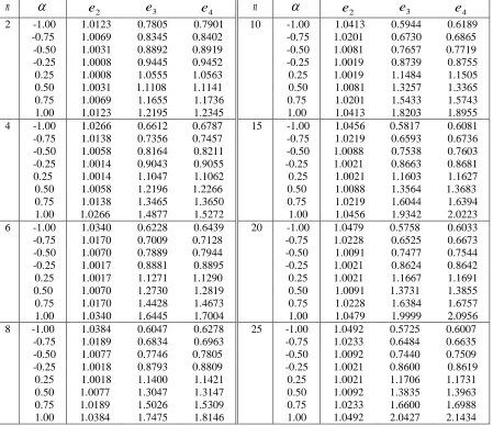
Table 1: The values of relative efficiencies e2,e3, and e4 in MTBRD
n
e2 e3 e4 n
e2 e3 e42 -1.00 1.0123 0.7805 0.7901 10 -1.00 1.0413 0.5944 0.6189 -0.75 1.0069 0.8345 0.8402 -0.75 1.0201 0.6730 0.6865 -0.50 1.0031 0.8892 0.8919 -0.50 1.0081 0.7657 0.7719 -0.25 1.0008 0.9445 0.9452 -0.25 1.0019 0.8739 0.8755
0.25 1.0008 1.0555 1.0563 0.25 1.0019 1.1484 1.1505
0.50 1.0031 1.1108 1.1141 0.50 1.0081 1.3257 1.3365
0.75 1.0069 1.1655 1.1736 0.75 1.0201 1.5433 1.5743
1.00 1.0123 1.2195 1.2345 1.00 1.0413 1.8203 1.8955
4 -1.00 1.0266 0.6612 0.6787 15 -1.00 1.0456 0.5817 0.6081
-0.75 1.0138 0.7356 0.7457 -0.75 1.0219 0.6593 0.6736 -0.50 1.0058 0.8164 0.8211 -0.50 1.0088 0.7538 0.7603 -0.25 1.0014 0.9043 0.9055 -0.25 1.0021 0.8663 0.8681
0.25 1.0014 1.1047 1.1062 0.25 1.0021 1.1603 1.1627
0.50 1.0058 1.2196 1.2266 0.50 1.0088 1.3564 1.3683
0.75 1.0138 1.3465 1.3650 0.75 1.0219 1.6044 1.6394
1.00 1.0266 1.4877 1.5272 1.00 1.0456 1.9342 2.0223
6 -1.00 1.0340 0.6228 0.6439 20 -1.00 1.0479 0.5758 0.6033 -0.75 1.0170 0.7009 0.7128 -0.75 1.0228 0.6525 0.6673
-0.50 1.0070 0.7889 0.7944 -0.50 1.0091 0.7477 0.7544
-0.25 1.0017 0.8881 0.8895 -0.25 1.0021 0.8624 0.8642
0.25 1.0017 1.1271 1.1290 0.25 1.0021 1.1667 1.1691
0.50 1.0070 1.2730 1.2819 0.50 1.0091 1.3731 1.3855
0.75 1.0170 1.4428 1.4673 0.75 1.0228 1.6384 1.6757
1.00 1.0340 1.6445 1.7004 1.00 1.0479 1.9999 2.0956
8 -1.00 1.0384 0.6047 0.6278 25 -1.00 1.0492 0.5725 0.6007
-0.75 1.0189 0.6834 0.6963 -0.75 1.0233 0.6484 0.6635
-0.50 1.0077 0.7746 0.7805 -0.50 1.0092 0.7440 0.7509
-0.25 1.0018 0.8793 0.8809 -0.25 1.0021 0.8600 0.8619
0.25 1.0018 1.1400 1.1421 0.25 1.0021 1.1706 1.1731
0.50 1.0077 1.3047 1.3147 0.50 1.0092 1.3835 1.3963
0.75 1.0189 1.5026 1.5309 0.75 1.0233 1.6600 1.6988
3. Estimating based on ERSS and MERSS
In this section, first we derive different estimators for
2based on ERSS method withconcomitant variable. This method introduced by Samawi et al. (1996) and can be described as follows:
Step 1. Select n random samples each of size n bivariate units from the population.
Step 2. If the sample size n is even, then select from
2
n
samples the smallest ranked unit
X together with the associated Yand from the other
2
n
samples the largest ranked unit
X together with the associated Y.This selected observations
,
(
),
,
(
),
,
(
X
(1)1Y
[1]1X
(n)2Y
[n]2X
(1)3Y
[1]3),
,
(
X
(1)n1,
Y
[1]n1),
(
X
(n)n,
Y
[n]n)
can be denoted by1
ERSS .
Step 3. If n is odd then select from
2 1
n
samples the smallest ranked unit X together
with the associated Y and from the other
2 1
n
samples the largest ranked unit X
together with the associated Y and from one sample the median of the sample for actual
measurement. In this case the selected observations
),
,
(
,
),
,
(
),
,
(
),
,
(
X
(1)1Y
[1]1X
(n)2Y
[n]2X
(1)3Y
[1]3
X
(n)n1Y
[n]n1 ) 2 , 2(X(1)nX(n)n Y[1]nY[n]n can
be denoted ERSS2 and
(
X
(1)1,
Y
[1]1),
(
X
(n)2,
Y
[n]2),
(
X
(1)3,
Y
[1]3),
)
,
(
),
,
(
,
] 2
1 [ ) 2
1 ( 1 ] [ 1 ) (
n n n n n
n n
n
Y
X
Y
X
can be denoted by ERSS3.Theorem 3.1 i. When n is even, an unbiased estimator for
2 using ERSS1 is), (
2 1 =
ˆ /2 [1]2 1 [ ]2
1 = 1
ERSS
2, r n r
n
r
Y Y
n
(3.1)
with the variance
), (1 ) (4 = ) ˆ (
2 2 1 ERSS
2, cn
n
Var
where )2
1 ) 2 1)(1 (
( ) 2(4 =
n
n
cn
ii. When n is odd, unbiased estimators for
2 using ERSS2 and ERSS3 are ), 2 1 2 1 ( 2 1 =ˆ [1]1 [ ]2 [1]3 [ ] 1 [1] [ ]
2 ERSS
2, Y Yn Y Ynn Y n Ynn
n ). ( 2 1 = ˆ ] 2 1 [ 1 ] [ [1]3 ]2 [ [1]1 3 ERSS 2, n n n n
n Y Y Y
Y Y n
with the variances
], ) 1)/ ( 4 (1 2 1 2 [ ) (4 = ) ˆ ( 2 2 2 ERSS
2, cn n n dn
n n n
Var
], 1)/ ( 4 [1 ) (4 = ) ˆ ( 2 2 3 ERSS2, c n n
n
Var n
respectively, where 2 2
2 2) ( 1) )( 2(4 3) )( 2 2 (3 = n n n
dn .
Proof. The proof is obvious.
The efficiency of ˆ2,RSS relative to the estimators
1 ERSS 2,
ˆ
, 2 ERSS 2,ˆ
and3 ERSS 2,
ˆ
, respectively, are , 1 1 = ) ˆ | ˆ (= 2,RSS
1 ERSS 2, 5 n n c b e e
, ) ) 1)/ ( 4 (1 2 1 2 1 = ) ˆ | ˆ (= 2,RSS
2 ERSS 2, 6 n n n d n n c n n b e e . 1)/ ( 4 1 1 = ) ˆ | ˆ (
= 2,RSS
3 ERSS 2, 7 n n c b e e n n
Note that 3 41ei for i=5,6,7. Also, for fixed n, ei's increase in
|
|
, and for fixed|
|
, ei's increase in n. Therefore,1 ERSS 2,
ˆ
, 2 ERSS 2,ˆ
and3 ERSS 2,
ˆ
are more efficient thanRSS 2,
ˆ
.
The concept of MERSS with concomitant variable is proposed by Saleh and Al-Ananbeh (2007) for estimation of means of the bivariate normal distribution. Here, we consider that the random vector (X,Y) has a MTBRD as defined in (1.1). The procedure
Step 1. Select n samples each of size n from MTBRD using SRS. Identify by judgment the minimum of each sample with respect to the variable X.
Step 2. Repeat step 1, but for the maximum.
Note that the 2n pairs of set
{(
X
(1)r,
Y
[1]r),
(
X
(n)r,
Y
[n]r);
r
=
1,2,
,
n
}
that are obtained using the above procedure, are independent but not identically distributed.Theorem 3.2 An unbiased estimator of
2 based on MERSS is given by), (
2 1 =
ˆ [1] [ ]
1 = MERSS
2, r nr
n
r
Y Y
n
(3.2)with the variance
). 2 1 ( ) (4 = ) ˆ ( 2 2 MERSS 2, n c n
Var
Proof. The proof is obvious.
The efficiency of
ˆ
2,RSS relative to
ˆ
2,MERSS is. 1 ) 2(1 = ) ˆ | ˆ (
= 2,MERSS 2,RSS
8 n n c b e e
Note that 3 81e8 . Thus,
ˆ
2,MERSS is more efficient than
ˆ
2,RSS. Also, the efficiency ofMERSS 2,
ˆ
relative to *2
and
~2 are, ) 2 1 ( 4 = ) ˆ | ( = 2 1 = MERSS 2, * 2 9 r r n r n c n e e
).
2
1
(
)
(4
=
)
ˆ
|
~
(
=
2 MERSS 2, 2 10 n n nc
e
e
The efficiency of 2* relative to the estimators
1 ERSS 2,
ˆ
, 2 ERSS 2,ˆ
and3 ERSS 2,
ˆ
areFinally, the efficiency of
~2 relative to1 ERSS 2,
ˆ
,2 ERSS 2,
ˆ
and3 ERSS 2,
ˆ
are, ) (1 ) (4 = ) ~ | ˆ (
= 2 2
1 ERSS 2, 14
n n
n
c e
e
, ] ) 4 (1 2
1 2 [ ) (4 = ) ~ | ˆ
( =
2 2
2 ERSS 2, 15
n n n
n
d c n
n e
e
. ) 1) 4( (1 ) (4 = ) ~ | ˆ
( =
2 2
3 ERSS 2, 16
n n
n
c n n e
e
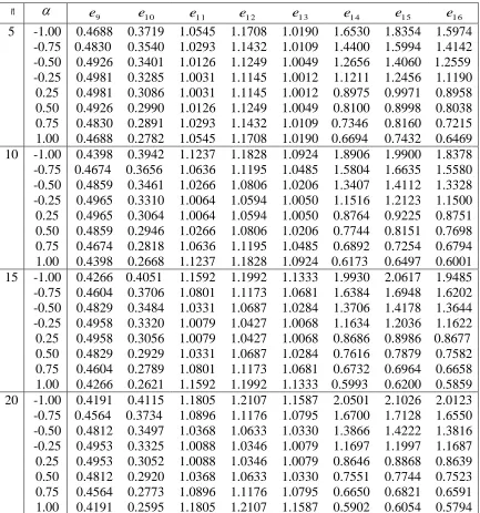
We computed the values of ej ,j=9,10,,16 for =0.25,0.5,0.75,1 and = 5(5)20.
n The results are given in Table 2, and we can conclude that
i) The efficiencies of ˆ2,MERSS relative to 2* and
~2 are less than 1 for n5. So,MERSS 2,
ˆ
is relatively more efficient than 2* and
~2.ii) The efficiencies of 2* relative to the estimators
1 ERSS 2,
ˆ
,2 ERSS 2,
ˆ
and3 ERSS 2,
ˆ
are morethan 1 for n5. Thus,
1 ERSS 2,
ˆ
,2 ERSS 2,
ˆ
and3 ERSS 2,
ˆ
are relatively more efficient than *2
.
iii) The efficiencies of
~2 relative to the estimators1 ERSS 2,
ˆ
,2 ERSS 2,
ˆ
and3 ERSS 2,
ˆ
are morethan (less than) 1 for 1 <0 (0<1) and n5. Thus
~2 is relatively more efficient than1 ERSS 2,
ˆ
,2 ERSS 2,
ˆ
and3 ERSS 2,
ˆ
when 0<1.4. Estimating based on DRERSS
In this section, first we obtain different estimators for
2 based on DRERSS method with concomitant variable. This method introduced by Al-Omari (2011) and can be described as follows:Step 1. Select n2 random samples each of size n bivariate units from the population.
Step 2. Select the coefficient k=[n], where 0< <1, and [x] is the largest integer value
Table 2: The values of ej for j=9,10,,16 in MTBRD
n
e9 e1 0 e11 e12 e1 3 e14 e1 5 e1 6 5 -1.00 0.4688 0.3719 1.0545 1.1708 1.0190 1.6530 1.8354 1.5974-0.75 0.4830 0.3540 1.0293 1.1432 1.0109 1.4400 1.5994 1.4142 -0.50 0.4926 0.3401 1.0126 1.1249 1.0049 1.2656 1.4060 1.2559 -0.25 0.4981 0.3285 1.0031 1.1145 1.0012 1.1211 1.2456 1.1190 0.25 0.4981 0.3086 1.0031 1.1145 1.0012 0.8975 0.9971 0.8958 0.50 0.4926 0.2990 1.0126 1.1249 1.0049 0.8100 0.8998 0.8038 0.75 0.4830 0.2891 1.0293 1.1432 1.0109 0.7346 0.8160 0.7215 1.00 0.4688 0.2782 1.0545 1.1708 1.0190 0.6694 0.7432 0.6469 10 -1.00 0.4398 0.3942 1.1237 1.1828 1.0924 1.8906 1.9900 1.8378
-0.75 0.4674 0.3656 1.0636 1.1195 1.0485 1.5804 1.6635 1.5580 -0.50 0.4859 0.3461 1.0266 1.0806 1.0206 1.3407 1.4112 1.3328 -0.25 0.4965 0.3310 1.0064 1.0594 1.0050 1.1516 1.2123 1.1500 0.25 0.4965 0.3064 1.0064 1.0594 1.0050 0.8764 0.9225 0.8751 0.50 0.4859 0.2946 1.0266 1.0806 1.0206 0.7744 0.8151 0.7698 0.75 0.4674 0.2818 1.0636 1.1195 1.0485 0.6892 0.7254 0.6794 1.00 0.4398 0.2668 1.1237 1.1828 1.0924 0.6173 0.6497 0.6001 15 -1.00 0.4266 0.4051 1.1592 1.1992 1.1333 1.9930 2.0617 1.9485 -0.75 0.4604 0.3706 1.0801 1.1173 1.0681 1.6384 1.6948 1.6202 -0.50 0.4829 0.3484 1.0331 1.0687 1.0284 1.3706 1.4178 1.3644 -0.25 0.4958 0.3320 1.0079 1.0427 1.0068 1.1634 1.2036 1.1622
0.25 0.4958 0.3056 1.0079 1.0427 1.0068 0.8686 0.8986 0.8677 0.50 0.4829 0.2929 1.0331 1.0687 1.0284 0.7616 0.7879 0.7582 0.75 0.4604 0.2789 1.0801 1.1173 1.0681 0.6732 0.6964 0.6658 1.00 0.4266 0.2621 1.1592 1.1992 1.1333 0.5993 0.6200 0.5859 20 -1.00 0.4191 0.4115 1.1805 1.2107 1.1587 2.0501 2.1026 2.0123 -0.75 0.4564 0.3734 1.0896 1.1176 1.0795 1.6700 1.7128 1.6550 -0.50 0.4812 0.3497 1.0368 1.0633 1.0330 1.3866 1.4222 1.3816 -0.25 0.4953 0.3325 1.0088 1.0346 1.0079 1.1697 1.1997 1.1687 0.25 0.4953 0.3052 1.0088 1.0346 1.0079 0.8646 0.8868 0.8639 0.50 0.4812 0.2920 1.0368 1.0633 1.0330 0.7551 0.7744 0.7523 0.75 0.4564 0.2773 1.0896 1.1176 1.0795 0.6650 0.6821 0.6591 1.00 0.4191 0.2595 1.1805 1.2107 1.1587 0.5902 0.6054 0.5794
Step 3. If n is even, from the first 2
2
n
samples select the (k1)th smallest unit X
together with the associated Y and from the second 2 2
n
samples the (nk)th smallest
unit X together with the associated Y. If n is odd, select from the first
2 1) (n n
samples
the (k1)th smallest unit X together with the associated Y, and from the next n
samples the
2 1
n
2 1) (n n
samples the (nk)th smallest ranked unit with the associated Y . This step
yield n samples each of size n.
Step 4. For the n samples obtained in Step 3, if n is even, select for actual measurement from the first
2
n
samples the (k1)th smallest ranked unit X together with the
associated Y and from the second
2
n
samples the (nk)th smallest ranked unit X
together with the associated Y. If n is odd, select from the first
2 1
n
samples the
1)
(k th smallest ranked unit X together with the associated Y , the median from the
next sample and from the last
2 1
n
samples the (nk)th smallest ranked unit X
together with the associated Y. This step yields one sample of size n units from the DRERSS data.
Theorem 4.1 i. When n is even, an unbiased estimator for
2 using DRERSS is] [
2 1 =
ˆ [ ]
2)/2 ( = 1] [ /2
1 = DRERSSE
2, n kr
n
n r r k n
r
Y Y
n
(4.1)
with the variance
), (1 ) (4 = ) ˆ
(
2 2 DRERSSE
2, wn
n
Var
where )2
1
) 2 1)(1 2
( ( ) 2(4 =
n
k n
wn
.
ii. When n is odd, an unbiased estimator for
2 using DRERSS is] [
2 1 =
ˆ [ ]
3)/2 ( = ] 2
1 [ 1] [ 1)/2 (
1 = DRERSSO
2, n k r
n
n r r n r k n
r
Y Y
Y
n
(4.2)
with the variance
), (1 ) (4 = ) ˆ
(
2 2 DRERSSO
2, zn
n
Var
where n
w
nn
n
z
=
1
.The efficiency of ˆ2,RSS relative to the estimator ˆ2,DRERSS is odd is n z b even is n w b e e n n n n 1 1 1 1 = ) ˆ | ˆ (
= 2,DRERSS 2,RSS
17 (4.3)
Note that 1e17 1.3. Thus, ˆ2,DRERSS is more efficient than ˆ2,RSS. The efficiency of DRERSS
2,
ˆ
relative to the estimator ˆ2,MERSS is
odd is n c z even is n c w e e n n n n 1 ) 2(1 1 ) 2(1 = ) ˆ | ˆ (
= 2,MERSS 2,DRERSS
18 (4.4)
Where 1e18 2. So, ˆ2,MERSS is more efficient than ˆ2,DRERSS. The efficiency of
DRERSS 2,
ˆ
relative to the estimators 2* and
~2 are
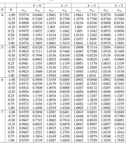
odd is n n z even is n n w e e r r n r n r r n r n 2 1 = 2 1 = DRERSS 2, * 2 19 ) )(4 (1 ) )(4 (1 = ) ˆ | ( = (4.5) odd is n n n z even is n n n w e e n n n n n n 2 2 DRERSS 2, 2 20 ) )(4 (1 ) )(4 (1 = ) ˆ | ~ ( = (4.6)We computed the values of e1 9 and e2 0 for
=
0.25,
0.5,
0.75,
1
, k0,1,2,3 and n4,5,6,7. The results are given in Table 3, and we can conclude that:i. The efficiency of ˆ2,DRERSS relative to 2* is less than 1 for k=0 and n4. So,
DRERSS 2,
ˆ
is relatively more efficient than 2*.
ii. The efficiency of ˆ2,DRERSS relative to the 2* is more than 1 for n5 and
k
=
1,2,3
. So, 2* is relatively more than efficient than ˆ2,DRERSS.iii. The efficiency of ˆ2,DRERSS relative to the
~2 is more than (less than) 1 for 0< 10)
<
1
Table 3: The values of e1 9 and e20 in MTBRD
k =0 k=1 k=2 k=3
n
e1 9 e20 e1 9 e20 e1 9 e20 e1 9 e20 4 -1.00 0.9576 0.6460 1.0661 0.7191 1.0661 0.7191 0.9576 0.6460-0.75 0.9768 0.7269 1.0357 0.7708 1.3578 0.7708 0.9768 0.7264 -0.50 0.9898 0.8136 1.0154 0.8346 1.0154 0.8346 0.9898 0.8136 -0.25 0.9975 0.9050 1.003 0.9107 1.003 0.9107 0.9975 0.9050
0.25 0.9975 1.0972 1.003 1.1042 1.003 1.1042 0.9975 0.9050 0.50 0.9898 1.1953 1.0154 1.2262 1.0154 1.2262 0.9898 1.1953 0.75 0.9768 1.2920 1.0357 1.3699 1.0357 1.3699 0.9768 1.2920 1.00 0.9576 1.3845 1.0661 1.5414 1.0661 1.5414 0.9576 1.3845 5 -1.00 0.9682 0.6320 1.0594 0.6916 1.0898 0.7114 1.0594 0.6916
-0.75 0.9824 0.7111 1.0318 0.7469 1.0483 0.7588 1.0318 0.7469 -0.50 0.9923 0.7996 1.0136 0.8168 1.0208 0.8226 1.0136 0.8168 -0.25 0.9981 0.8962 1.0033 0.9009 1.0051 0.9025 1.003 0.9009 0.25 0.9981 1.1101 1.0033 1.1159 1.0051 1.1179 1.0033 1.1159 0.50 0.9923 1.2258 1.0136 1.2521 1.0208 1.2609 1.0136 1.2521 0.75 0.9824 1.3460 1.0318 1.4136 1.0483 1.4362 1.0318 1.4136 1.00 0.9682 1.4695 1.0594 1.6080 1.0898 1.6541 1.0594 1.6080 6 -1.00 0.9215 0.5890 1.0339 0.6609 1.0902 0.6968 1.0902 0.6968 -0.75 0.9572 0.6799 1.0179 0.7230 1.0482 0.7445 1.0482 0.7445 -0.50 0.9814 0.7800 1.0076 0.8008 1.0207 0.8112 1.0207 0.8112 -0.25 0.9954 0.8873 1.0018 0.8930 1.0050 0.8959 1.0050 0.8959
0.25 0.9954 1.1159 1.0018 1.1231 1.0050 1.1267 1.0050 1.1267 0.50 0.9814 1.2324 1.0076 1.2653 1.0207 1.2818 1.0207 1.2818 0.75 0.9572 1.3456 1.0179 1.4309 1.0482 1.4735 1.0482 1.4735 1.00 0.9215 1.4498 1.0339 1.6268 1.0902 1.7153 1.0902 1.7153 7 -1.00 0.9359 0.5896 1.0287 0.6481 1.0843 0.6831 1.1029 0.6948 -0.75 0.9650 0.6761 1.0149 0.7110 1.0448 0.7320 1.0548 0.7390 -0.50 0.9847 0.7747 1.0062 0.7916 1.0192 0.8018 1.0235 0.8051 -0.25 0.9962 0.8832 1.0015 0.8878 1.0047 0.8907 1.0057 0.8916 0.25 0.9962 1.1235 1.0015 1.1295 1.0047 1.1331 1.0057 1.1343 0.50 0.9847 1.2522 1.0062 1.2795 1.0192 1.2959 1.0235 1.3014 0.75 0.9650 1.3834 1.0149 1.4550 1.0448 1.4979 1.0548 1.5122 1.00 0.9359 1.5139 1.0287 1.6639 1.0843 1.7539 1.1029 1.7839
5. An application
A reappraisal of caloric requirements in healthy women are done by Owen et al. (1986). The results of this study show that the body weight of women was highly related to the resting metabolic rate (RMR) of the women.
We considered a bivariate data set from the 44 women data such that the first component
6 from 44 women data and ranked the sampling units of each sample according to the X
variate (body weight). We measureed the ranked set sample observations Y[r]r
corresponding to X(r)r. The obtained RSS, ERSS1 and MERSS observations are given in
Table 4. Since the sample correlation coefficient is
3 1 >
q , the estimate for
is 1 (seeRemark 2.1).
The computed values of ˆ2,RSS,
1 ERSS 2,
ˆ
,ˆ2,MERSS are 1142.57, 1009.32, and 979.40,respectively. We can find that the estimated values for
2 based on different samplings are close.Table 4: Obtained RSS, ERSS1 and MERSS observations
r
1 2 3 4 5 6RSS X(r)r 49.9 48.1 56 62.1 82 99.8
r r
Y[ ] 1079 1372 1392 1574 1536 1639
1
ERSS X(1)2r1 49.9 55 66.4 1
[1]2r
Y 1079 1034 1205
r n
X( )2 64.9 66 99.8
r n
Y[ ]2 1365 1268 1639
MERSS X(1)r 49.9 43.1 55 59.2 66.4 83.4
r
Y[1] 1079 870 1034 1342 1205 1248
r n
X( ) 61.4 64.9 59 66 82 99.8
r n
Y[ ] 1351 1365 1178 1268 1151 1639
References
1. Al-Odat, M. and Al-Saleh, M.F. (2001). A variation of ranked set sampling. Journal of Applied Statistical Science, 10(2), 137–146.
2. Al-Omari, A.I. (2011). Estimation of mean based on modified robust extreme ranked set sampling. Journal of Statistical Computation and Simulation, 81(8), 1055–1066.
3. Al-Saleh, M. F. and Al-Ananbeh, A. M. (2005). Estimating the correlation coefficient in a bivariate normal distribution using moving extreme ranked set sampling with a concomitant variable. Journal of the Korean Statistical Society, 34(2), 125–140.
5. Al-Saleh, M. F. and Diab, Y. A. (2009). Estimation of the parameters of Downton's bivariate exponential distribution using ranked set sampling scheme. Journal of Statistical Planning and Inference, 139(2), 277–286.
6. Bairamov, I. and Bekci, M. (1999). Concomitant of order statistics in fgm type bivariate uniform distributions. Istatistik, Journal of the Turkish Statistical Association, 2(2), 135–144.
7. Balasubramanian, K. and Beg, M. I. (1997). Concomitants of order statistics in Morgenstern type bivariate exponential distribution. Journal of Applied Statistical Science, 54(4), 233–245.
8. Chacko, M. and Thomas, P. Y. (2008). Estimation of a parameter of Morgenstern type bivariate exponential distribution by ranked set sampling. Annals of the Institute of Statistical Mathematics, 60(2), 301–318.
9. Chacko, M. and Thomas, P. Y. (2011). Estimation of parameter of Morgenstern type bivariate exponential distribution using concomitants of order statistics. Statistical Methodology, 8(4), 363–376.
10. David, H. A. and Nagaraja, H. (2003). Order Statistics. John Wiley and Sons.
11. D'Este, G. (1981). A Morgenstern-type bivariate gamma distribution. Biometrika, 68(1), 339–340.
12. Farlie, D. J. G. (1960). The performance of some correlation coefficients for a general bivariate distribution. Biometrika, 47(3/4), 307–323.
13. Gumbel, E. J. (1960). Bivariate exponential distributions. Journal of the American Statistical Association, 55(292), 698–707.
14. Gumbel, E. J. (1961). Bivariate logistic distributions. Journal of the American Statistical Association, 56(294), 335–349.
15. Lam, K., Sinha, B. K., and Wu, Z. (1994). Estimation of parameters in a two-parameter exponential distribution using ranked set sample. Annals of the Institute of Statistical Mathematics, 46(4), 723–736.
16. McIntyre, G. A. (1952). A method for unbiased selective sampling, using ranked sets. Australian Journal of Agricultural Research, 3(4): 385–390.
17. Morgenstern, D. (1956). Einfache beispiele zweidimensionaler verteilungen. Mitteilingsblatt für Mathematishe Statistik, 8(1), 234–235.
18. Owen, O. E., Kavle, E., Owen, R. S., Polansky, M., Caprio, S., Mozzoli, M. A., Kendrick, Z. V., Bushman, M., and Boden, G. (1986). A reappraisal of caloric requirements in healthy women. The American Journal of Clinical Nutrition, 44(1), 1–19.
19. Samawi, H. M., Ahmed, M. S., and Abu-Dayyeh, W. (1996). Estimating the population mean using extreme ranked set sampling. Biometrical Journal, 38(5): 577–586.
21. Singh, H. P and Mehta.V (2015). Estimation of scale parameter of a Morgenstern type bivariate uniform distribution using censored ranked set samples. Model Assisted Statistics and Applications, 10(2), 139–153.
22. Stokes, S. L. (1977). Ranked set sampling with concomitant variables. Communications in Statistics - Theory and Methods, 6(12), 1207–1211.
23. Stokes, S. L. (1980). Inferences on the correlation coefficient in bivariate normal populations from ranked set samples. Journal of the American Statistical Association, 75(372), 989–995.
24. Stokes, S. L. (1995). Parametric ranked set sampling. Annals of the Institute of Statistical Mathematics, 47(3), 465–482.
25. Tahmasebi, S. and Jafari, A. A. (2012). Estimation of a scale parameter of Morgenstern type bivariate uniform distribution by ranked set sampling. Journal of Data Science, 10, 129–141.
26. Tahmasebi, S. and Jafari, A. A. (2015). Concomitants of order statistics and record values from Morgenstern type bivariate generalized exponential distribution. Bulletin of the Malaysian Mathematical Sciences Society, 38(4), 1411–1423.
27. Tahmasebi, S. and Jafari, A. A. (2014). Estimators for the parameter mean of Morgenstern type bivariate generalized exponential distribution using ranked set sampling. Statistics and Operations Research Transactions, 38(2), 161–180.