Application of Blind Deconvolution
Algorithm for Image Restoration
D. SRINIVASA RAO
Faculty of Computer Science Applications Anil Neerukonda Institute of Technology & Sciences
Visakhapatnam, India
K. SELVANI DEEPTHI
Faculty of Computer Science Engineering Anil Neerukonda Institute of Technology & Sciences
Visakhapatnam, India
K. MONI SUSHMA DEEP
Faculty of Computer Science Applications Anil Neerukonda Institute of Technology & Sciences
Visakhapatnam, India
Abstract:
Image restoration is the process of recovering the original image from the degraded image and also understand the image without any artifacts errors. Image restoration methods can be considered as direct techniques when their results are produced in a simple one step fashion. Equivalently, indirect techniques can be considered as those in which restoration results are obtained after a number of iterations. Known restoration techniques such as inverse filtering and Wiener Filtering can be considered as simple direct restoration techniques. The problem with such methods is that they require knowledge of the blur function that is point-spread function (PSF), which is, unfortunately, usually not available when dealing with image blurring . In this paper Blind deconvolution for image restoration is discussed which is the recovery of a sharp version of a blurred image when the blur kernel is unknown.
The fundamental task of image deblurring is to de-convolute the blurred/degraded image with the PSF that exactly describes the distortion. Firstly, the original image is degraded using the Degradation Model. It can be done by Gaussian Filter which is low-pass filter used to blur in image. In the edges of degraded image, the ringing effect due to high frequency drop-off can be detected using Canny Edge detection methods. This ringing effect should be removed before restoration using edge trapping. After removing the ringing effect, blind Deconvolution algorithm is applied to the blurred images. It is possible to renovate the original image without having specific knowledge of degradation filter, additive noise and image spectral density. Recent algorithms have afforded dramatic progress, yet many aspects of the problem remain challenging and hard to understand. The goal of this paper is to analyze and evaluate recent blind deconvolution algorithms both theoretically and experimentally.
Keywords- Blind Deconvolution Algorithm, Canny Edge Detection, Degradation Model, Image Restoration, PSF
1. Introduction
Blurring is a form of bandwidth reduction of the image due to imperfect image formation process. It can be caused by relative motion between camera and original images. Normally, an image can be degraded using low-pass filters and its noise. This low-pass filter is used to blur/smooth the image using certain functions.
1.1 Blurring Types
In digital image there are 3 common types of Blur effects[1]:
Gaussian Blur
Motion Blur
1.1.1. Average Blur
The Average blur is one of several tools we can use to remove noise and specks in an image. Use it when noise is present over the entire image. This type of blurring can be distribution in horizontal and vertical direction and can be circular averaging by radius R which is evaluated by the formula:
R =√ g2 + f2
Where: g is the horizontal size blurring direction and f is vertical blurring size direction and R is the radius size of the circular average blurring.
1.1.2. Gaussian Blur
The Gaussian Blur effect is a filter that blends a specific number of pixels incrementally, following a bell-shaped curve. The blurring is dense in the center and feathers at the edge. Apply Gaussian Blur to an image when we want more control over the Blur effect.
1.1.3. Motion Blur
The Motion Blur effect is a filter that makes the image appear to be moving by adding a blur in a specific direction. The motion can be controlled by angle or direction (0 to 360 degrees or –90 to +90) and/or by distance or intensity in pixels (0 to 999), based on the software used.
1.2. Deblurring
1.2.1. Why Deblurring
• Better looking image • Improved identification
Reduces overlap of image structure to more easily identify features in the image (needs high SNR)
• PSF calibration
Removes artifacts in the image due to the point spread function (PSF) of the system, i.e. extended halos, lumpy Airy rings etc.
• Higher resolution
In specific cases depending upon algorithms and SNR
Better Quantitative Analysis
1.2.2. Deblurring Model
A blurred or degraded image can be approximately described by this equation:
g = PSF*f + N, Where: g the blurred image, h the distortion operator called Point Spread Function (PSF), f the original true image and N Additive noise, introduced during image acquisition, that corrupts the image[1].
Point Spread Function (PSF)
Point Spread Function (PSF) is the degree to which an optical system blurs (spreads) a point of light. The PSF is the inverse Fourier transform of Optical Transfer Function (OTF).in the frequency domain ,the OTF describes the response of a linear, position-invariant system to an impulse.OTF is the Fourier transfer of the point (PSF).
Image deblurring is an inverse problem which is used to recover an image which has suffered from linear degradation. The blurring degradation can be space-invariant or space-in variant[2]. Image deblurring methods can be divided into two classes: nonblind, in which the blurring operator is known and blind, in which the blurring operator is unknown.
1.3.1. Non Blind image deblurring technique:
i). Wiener Filter Deblurring Technique
The Wiener filter isolates lines in a noisy image by finding an optimal tradeoff between inverse filtering and noise smoothing. It removes the additive noise and inverts the blurring simultaneously so as to emphasize any lines which are hidden in the image. This filter operates in the Fourier domain[4], making the elimination of noise easier as the high and low frequencies are removed from the noise to leave a sharp image. Using Fourier transforms means the noise is easier to completely eliminate and the actual line embedded in noise easier to isolate making it a slightly more effective method of filtering. The Wiener filter in Fourier domain can be expressed as follows:
Where are respectively the power spectra of the original image and the additive noise, and H(f1,f2) is the blurring filter. Here one can see that the Wiener filter has two separate parts, an inverse filtering part and a noise smoothing part. It not only performs the deconvolution by inverse filtering (high pass filtering) but also removes the noise with low pass filtering.
ii). Regularized Filter Deblurring Technique
Regulated filter is the deblurring method to deblur an Image by using deconvlution function deconverge which is effective when the limited information is known about additive noise
• Reparameterization of the object with a smoothing kernel – (sieve function or low-pass filter). F(r ) = Ø(r )2 * a(r )
• Truncated iterations
stop convergence when the error-metric reaches the noise-limit, gi=g ’
i+ni , such that ENσ 2
n
iii). Lucy-Richardson Algorithm Technique
Discrete Convolution[8,9]
From Bayes theorem P(gi|fj) = hij and the object distribution can be expressed iteratively as
so that the LR kernel approaches unity as the iterations progress
1.3.2. Blind image deblurring technique
Blind Deconvolution is a subset of Iterative Constrained algorithms which produce an estimate of h(x) concurrently with f(x)[3]. It does not need the PSF h(x) to be measured. Other iterative constrained algorithms require h(x) to be measured by acquiring data from subresolution fluorescent beads.
g(x) = f(x)*h(x)+n(x)
where
g(x): measurement f(x): unknown object
h(x): unknown or poorly known PSF n(x): contamination
The algorithm is producing the PSF from information within the data set g(x). This is done by first assuming an h(x), then (1), estimating which f(x) could have caused g(x). This calculation is followed by (2), estimating which h(x) could have caused g(x) from the estimated f(x), and then steps (1) and (2) are repeated again and again. It is believable that the PSF information is in the data because one often sees the light spreading from fine point or line structures in the data, and this spreading makes up the PSF.
The rest of the paper structured as follows: Section 2 describes the degradation model and also parameters required for blurring the image. Section 3 describes application of Canny Edge Detection and ringing effect to detect an edge of the image. Section 4 shows the over all architecture of deblurring the image. Section 5 describe about the proposed algorithm used for deblurring the image. Section 6 shows the sample result of blurred and deblurred of original image using our proposed algorithm. In section 7 we conclude the paper having future scope.
2. Image Degradation Model
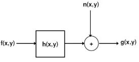
In the model of image degradation [5] fig. 1, the observed image g(x, y) is modeled as the output of a 2-D linear system and can be characterized by its degradation function h(x, y). The noise n(x, y) is assumed to be a Gaussian white noise with zero mean. If the degradation function h(x, y) is linear and space invariant function, then the observed blurred/noisy image in spatial domain is given by
G(x, y) =h(x, y)*f(x, y) + n(x, y)
Fig. 1: Image Degradation Model
2.1. Gaussian Filter
Gaussian filter is used to blur an image using Gaussian function [10]. It requires two parameters such as mean and variance. It is weighted blurring. Gaussian functions of the following from
G(x, y) =1/2 πσ2 * e-x2+y2/2σ2
Where σ is variance and x and y are the distance from the origin in the horizontal axis and vertical axis respectively. Gaussian Filter has an efficient implementation of that allows it to create a very blurry blur image in relatively short time.
2.2. Gaussian Noise
The ability to simulate the behavior and effects of noise is central to image restoration. Gaussian noise is a white noise with constant mean and variance which is represented by a series of outputs Yi at discrete time event index i[10]. Yi is the sum of the input Xi and noise, Zi, where Zi is independent and identically-distributed and drawn from a zero-mean normal distribution with variance n (the noise). The Zi are further assumed to not be correlated with the Xi. The default values of mean and variance are 0 and 0.01 respectively.
Yi = Xi + Zi
2.3. Blurring Parameter
The parameters needed for blurring an image are PSF, Blur length, Blur angle and type of noise. Point Spread Function is a blurring function. When the intensity of the observed point image is spread over several pixels, this is known as PSF. Blur length is the number of pixels by which the image is degraded. It is number of pixel position is shifted from original position. Blur angle is an angle at which the image is degraded. Available types of noise are Gaussian noise, salt and pepper noise, Poisson noise, Speckle noise which is used for blurring. In this paper, we are using Gaussian noise which is also known as white noise. It requires mean and variance as parameters.
2.4. Algorithm for Degradation Model Input Input:
Load and input image ‘f’ Initialize blur length ‘I’
Initialize blur angle ‘theta’ Assign The type of noise ‘n’
PSF (Point Spread Function), ‘h’
Procedure- I
H=create (f, 1, theta) % Creation of PSF Blurred image (g) =f*h+n
G=filter (f, h, n, “convolution”) If ‘g’ contains “ringing” at its edge then
Remove ringing effect using edge taper function Else
Go to Procedure – II End Procedure – I
3. Candy Edge Detection and Ringing Effect
The Discrete Fourier Transform used by the deblurring function creates high frequency drop-off at the edges of images. This high frequency drop-off at the edges of images. This high frequency drop-off can create an effect called boundary related ringing in deblurred images. For avoiding this ringing effect at the edge of image, we have to detect the edge of an image. There are various edge detection methods available to detect an edge of the image.
The edge can be detected effectively using Canny Edge Detection methods. It differs from to other edge-detection methods such as Sobel, Prewitt, Roberts, Log in that it uses two different thresholds for detecting both strong and weak edges. Edge provides a number of derivative (of the intensity is larger than threshold) estimators.
3.1. Candy Edge Detector
Canny edge detection methods find edges by looking for local maxima of the gradient of (x, y). The gradient is calculated using the derivate of a Gaussian Filter. The method uses two thresholds to detect strong and weak edges, and includes the weak edges in the output only if they are connected to strong edges. Therefore, this method is more likely to detect true weak edges.
Steps involved in canny methods:
The image is smoothed using Gaussian Filter with a specified standard deviation, σ to reduce noise
The local gradient, g(x, y) and edge direction are computed at each point.
The edge point determined give rise to ridges in the gradient magnitude image. This ridge pixels are then thresholds, T1 and T2, with T1<T2.
3.2. Edge taper for Ringing Effect
The ringing effect can be avoided using edge taper function. Edge taper function is used to preprocess our image before passing it to the deblurring functions. It removes the high frequency drop-off at the edge of an image by blurring the entire image & then replacing the center pixels of the blurred image with the original image ie.
J = edgetaper (I, PSF) blurs the edges of the input image, I, using the point spread function, PSF. The output image, J, is the weighted sum of the original image, I, and its blurred version [7]. The weighting array, determined by the autocorrelation function of PSF, makes J equal to I in its central region, and equal to the blurred version of I near the edges.
The edgetaper function reduces the ringing effect in image deblurring methods that use the discrete Fourier transform.
4. Architecture of Deblurring the Image
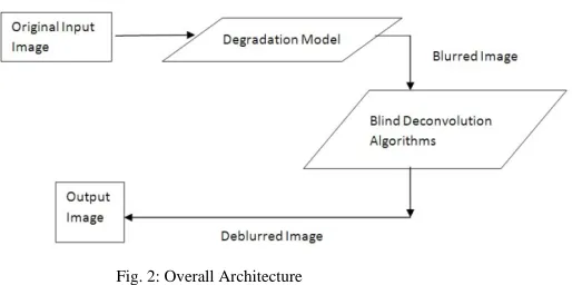
Fig. 2: Overall Architecture
The original image is degraded or blurred using degradation model to produce the blurred image. The blurred image should be an input to the deblurring algorithm. Various algorithms are available for deblurring. In this paper, we are going to use blind deconvolution algorithm. The result of this algorithm produces the deblurring image which can be compared with our original image.
5. Blind Deconvolution Algorithm
Blind Deconvolution Algorithm can be used effectively when no information of distortion is known; it restores image and PSF simultaneously. This algorithm can be achieved based on Maximum Likelihood Estimation (MLE).
Algorithm for Deblurring Input:
Blurred image ‘g’ Initialize number of iterations ‘i’ Initial PSF ‘h’
Weight of an image ‘w’ % pixels considered for restoration a=0 (default) % Array corresponding to additive noise
Procedure-II
If PSF is not known then
Guess initial values of PSF Else
Specify the PSF of degraded image Restored Image f= Deconvolution (g, h, i, w, a)
End Procedure- II 6. Sample Results
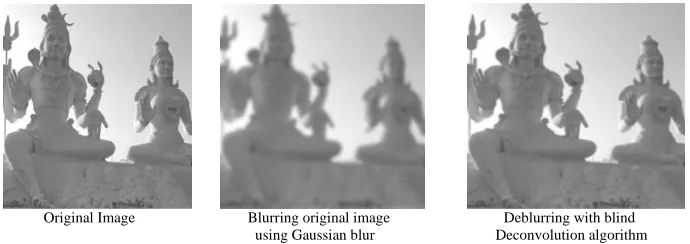
Original Image Blurring original image Deblurring with blind using Gaussian blur Deconvolution algorithm
Fig. 3: Deblurring image with no information of PSF
7. Conclusion
We have presented a method for blind image deblurring. The method differs from most other existing methods by only imposing weak restrictions on the blurring filter, being able to recover images which have suffered a wide range of degradations. Good estimates of both the image and the blurring operator are reached by initially considering the main image edges. The restoration quality of our method was visually and quantitatively better than those of the other algorithms such as wiener Filter algorithms, Regularization algorithm and Lucy Richardson with which it was compared. The advantage of our proposed Blind Deconvoultion algorithm is used to deblur the degraded image without prior knowledge of PSF and additive noise. But in other algorithms, we should have the knowledge over the blurring parameters.
The future work of this paper is to increase the speed of the deblurring process that is reducing the number of iteration using for deblurring the image for achieving better quality image.
References
[1] Salem Saleh Al-amri et. al. “A Comparative Study for Deblured Average Blurred Images “,journal Vol. 02, No. 03, 2010, 731-733. [2] Michal Sorel and Jan Flusser, Senior Member, IEEE., Space-Variant Restoration of Images Degraded by Camera Motion Blur, IEEE
Transaction on image processing, Vol 17, pp.105-116, No. 2 Febreary 2008.
[3] Jain-feng cai, hui ji, Chaoqiang lie, Zuowei Shen., “blind Motion deblurring using multiple images”. Journal of Computation Physics. Pp. 5057-5071, 2009.
[4] J. Goodman, “Introduction to Fourier Optics”, McGraw Hill, 1996.
[5] D. Kundur and D. Hatziankos, “Blind image deconvolution, “ IEEE sig. process. Mag., pp. 43-64, May 1996.
[6] Rafael C. Gonzalex, Richard E. Woods, Steven L. Eddins, Digital Image Processing Using MATLAB (Persona Education, Inc., 2006). [7] Mariana S.C. Almeida and Luis B. Almeida., Blind and Semi-Blind Deblurring of Natural Images, IEEE Transaction on Image
processing, Vol 19, pp.36-52, No.1, January 2010.