https://doi.org/10.5194/amt-12-5161-2019 © Author(s) 2019. This work is distributed under the Creative Commons Attribution 4.0 License.
Gaussian process regression model for dynamically calibrating
and surveilling a wireless low-cost particulate matter
sensor network in Delhi
Tongshu Zheng1, Michael H. Bergin1, Ronak Sutaria2, Sachchida N. Tripathi3, Robert Caldow4, and David E. Carlson1,5
1Department of Civil and Environmental Engineering, Duke University, Durham, NC 27708, USA
2Respirer Living Sciences Pvt. Ltd, 7, Maheshwar Nivas, Tilak Road, Santacruz (W), Mumbai 400054, India 3Department of Civil Engineering, Indian Institute of Technology Kanpur, Kanpur, Uttar Pradesh 208016, India 4TSI Inc., 500 Cardigan Road, Shoreview, MN 55126, USA
5Department of Biostatistics and Bioinformatics, Duke University, Durham, NC 27708, USA
Correspondence:Tongshu Zheng ([email protected]) Received: 11 February 2019 – Discussion started: 1 March 2019
Revised: 19 July 2019 – Accepted: 30 August 2019 – Published: 26 September 2019
Abstract. Wireless low-cost particulate matter sensor net-works (WLPMSNs) are transforming air quality monitor-ing by providmonitor-ing particulate matter (PM) information at finer spatial and temporal resolutions. However, large-scale WLPMSN calibration and maintenance remain a challenge. The manual labor involved in initial calibration by colloca-tion and routine recalibracolloca-tion is intensive. The transferability of the calibration models determined from initial collocation to new deployment sites is questionable, as calibration fac-tors typically vary with the urban heterogeneity of operating conditions and aerosol optical properties. Furthermore, the stability of low-cost sensors can drift or degrade over time. This study presents a simultaneous Gaussian process regres-sion (GPR) and simple linear regresregres-sion pipeline to calibrate and monitor dense WLPMSNs on the fly by leveraging all available reference monitors across an area without resorting to pre-deployment collocation calibration. We evaluated our method for Delhi, where the PM2.5measurements of all 22
regulatory reference and 10 low-cost nodes were available for 59 d from 1 January to 31 March 2018 (PM2.5averaged
138±31 µg m−3among 22 reference stations), using a leave-one-out cross-validation (CV) over the 22 reference nodes. We showed that our approach can achieve an overall 30 % prediction error (RMSE: 33 µg m−3) at a 24 h scale, and it
is robust as it is underscored by the small variability in the GPR model parameters and in the model-produced calibra-tion factors for the low-cost nodes among the 22-fold CV. Of
the 22 reference stations, high-quality predictions were ob-served for those stations whose PM2.5means were close to
the Delhi-wide mean (i.e., 138±31 µg m−3), and relatively poor predictions were observed for those nodes whose means differed substantially from the Delhi-wide mean (particularly on the lower end). We also observed washed-out local vari-ability in PM2.5 across the 10 low-cost sites after
5162 T. Zheng et al.: Gaussian process regression model
calibration. Simulations conducted using our algorithm sug-gest that in addition to dynamic calibration, the algorithm can also be adapted for automated monitoring of large-scale WLPMSNs. In these simulations, the algorithm was able to differentiate malfunctioning low-cost nodes (due to ei-ther hardware failure or under the heavy influence of local sources) within a network by identifying aberrant model-generated calibration factors (i.e., slopes close to zero and intercepts close to the Delhi-wide mean of true PM2.5). The
algorithm was also able to track the drift of low-cost nodes accurately within 4 % error for all the simulation scenarios. The simulation results showed that ∼20 reference stations are optimum for our solution in Delhi and confirmed that low-cost nodes can extend the spatial precision of a network by decreasing the extent of pure interpolation among only reference stations. Our solution has substantial implications in reducing the amount of manual labor for the calibration and surveillance of extensive WLPMSNs, improving the spa-tial comprehensiveness of PM evaluation, and enhancing the accuracy of WLPMSNs.
1 Introduction
Low-cost air quality (AQ) sensors that report high time res-olution data (e.g., ≤1 h) in near real time offer excellent potential for supplementing existing regulatory AQ monitor-ing networks by providmonitor-ing enhanced estimates of the spa-tial and temporal variabilities of air pollutants (Snyder et al., 2013). Certain low-cost particulate matter (PM) sensors have demonstrated satisfactory performances when benchmarked against Federal Equivalent Methods (FEMs) or research-grade instruments in some previous field studies (Holstius et al., 2014; Gao et al., 2015; SCAQMD, 2015a–c, 2017a–c; Jiao et al., 2016; Kelly et al., 2017; Mukherjee et al., 2017; Crilley et al., 2018; Feinberg et al., 2018; Johnson et al., 2018; Zheng et al., 2018). Application-wise, low-cost PM sensors have had success in identifying urban fine particle (PM2.5, with a diameter of 2.5 µm and smaller) hotspots in
Xi’an, China (Gao et al., 2015), mapping urban air quality with additional dispersion model information in Oslo, Nor-way (Schneider et al., 2017), monitoring smoke from pre-scribed fire in Colorado, US (Kelleher et al., 2018), measur-ing a traveler’s exposure to PM2.5in various
microenviron-ments in Southeast Asia (Ozler et al., 2018), and building up a detailed city-wide temporal and spatial indoor PM2.5
expo-sure profile in Beijing, China (Zuo et al., 2018).
On the down side, researchers have been plagued by calibration-related issues since the emergence of low-cost AQ sensors. One common brute force solution is initial cal-ibration by collocation with reference analyzers before field deployment and follow-up with routine recalibration. Yet, the transferability of these pre-determined calibrations at collo-cation sites to new deployment sites is questionable as
cali-bration factors typically vary with operating conditions such as PM mass concentrations, relative humidity (RH), temper-ature, and aerosol optical properties (Holstius et al., 2014; Austin et al., 2015; Wang et al., 2015; Lewis and Edwards, 2016; Crilley et al., 2018; Jayaratne et al., 2018; Zheng et al., 2018). Complicating this further, the pre-generated calibra-tion curves may only apply for a short term as the stability of low-cost sensors can develop drift or degrade over time (Lewis and Edwards, 2016; Jiao et al., 2016; Hagler et al., 2018). Routine recalibrations which require frequent transit of the deployed sensors between the field and the reference sites are not only too labor intensive for a large-scale network but also still cannot address the impact of urban heterogene-ity of ambient conditions on calibration models (Kizel et al., 2018).
As such, calibrating sensors on the fly while they are de-ployed in the field is highly desirable. Takruri et al. (2009) showed that the interacting multiple model (IMM) algo-rithm combined with the support vector regression (SVR)– unscented Kalman filter (UKF) can automatically and suc-cessfully detect and correct low-cost sensor measurement er-rors in the field; however, the implementation of this algo-rithm still requires pre-deployment calibrations. Fishbain and Moreno-Centeno (2016) designed a self-calibration strategy for low-cost nodes with no need for collocation by exploit-ing the raw signal differences between all possible pairs of nodes. The learned calibrated measurements are the vectors whose pairwise differences are closest in the normalized pro-jected Cook–Kress (NPCK) distance to the corresponding pairwise raw signal differences given all possible pairs over all time steps. However, this strategy did not include ref-erence measurements in the self-calibration procedure, and therefore the tuned measurements were still essentially raw signals (although instrument noise was dampened). An al-ternative calibration method involves chain calibration of the low-cost nodes in the field with only the first node calibrated by collocation with reference analyzers and the remaining nodes calibrated sequentially by their respective previous node along the chain (Kizel et al., 2018). While this node-to-node calibration procedure proved its merits in reducing collocation burden and data loss during calibration, reloca-tion, and recalibration and accommodating the influence of urban heterogeneity on calibration models, it is only suitable for relatively small networks because calibration errors prop-agate through chains and can inflate toward the end of a long chain (Kizel et al., 2018).
In this paper, we introduce a simultaneous Gaussian pro-cess regression (GPR) and simple linear regression pipeline to calibrate PM2.5 readings of any number of low-cost PM
interpolation (e.g., Holdaway, 1996; Di et al., 2016; Schnei-der et al., 2017), and the simple linear regression calibration can adjust for disagreements between the low-cost sensor and reference instrument measurements, leading to more consis-tent spatial interpolation. This paper focuses on the follow-ing:
1. quantifying experimentally the daily performance of our dynamic calibration model in Delhi during the win-ter season based on model prediction accuracy on the holdout reference nodes during leave-one-out cross-validations (CVs) and low-cost node calibration accu-racy;
2. revealing the potential pitfalls of employing a dynamic calibration algorithm;
3. examining the sensitivity of our algorithm to the train-ing data size and the feasibility of it for dynamic cali-bration;
4. demonstrating the ability of our algorithm to auto-detect faulty nodes and auto-correct the drift of nodes within a network via computational simulation, and therefore the practicality of adapting our algorithm for automated large-scale sensor network monitoring; and
5. studying computationally the optimal number of refer-ence stations across Delhi to support our technique and the usefulness of low-cost sensors for extending the spa-tial precision of a sensor network.
To the best of our knowledge, this is the first study to apply such a non-static calibration technique to a wireless low-cost PM sensor network in a heavily polluted region such as India and is the first to present methods of auto-monitoring dense AQ sensor networks.
2 Materials and methods 2.1 Low-cost node configuration
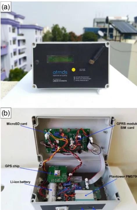
The low-cost packages used in the present study (dubbed “Atmos”) shown in Fig. 1a were developed by Respirer Living Sciences (http://atmos.urbansciences.in/, last access: 30 November 2018) and cost USD∼ 300 per unit. The Atmos monitor measures 20.3 cm L×12.1 cm W×7.6 cm H, weighs 500 g, and is housed in an IP65 (Ingress Pro-tection rating 65) enclosure with a liquid crystal display (LCD) on the front showing real-time PM mass concentra-tions and various debugging messages. It includes a Plan-tower PMS7003 sensor (USD∼ 25; dimension: 4.8 cm L
×3.7 cm W×1.2 cm H) to measure PM1, PM2.5, and PM10
mass concentrations, an Adafruit DHT22 sensor to mea-sure temperature and relative humidity, and an ultra-compact Quectel L80 GPS model to retrieve accurate locations in real time. The operating principle and configuration of PMS7003
are similar to its PMS1003, PMS3003, and PMS5003 coun-terparts and have been extensively discussed in previous studies (Kelly et al., 2017; Zheng et al., 2018; and Sayahi et al., 2019, respectively). The inlet and outlet of PMS7003 were aligned with two slots on the box to ensure unrestricted airflow into the sensor. The PM and meteorology data are read over the serial TTL interface every 3 seconds, aggre-gated every 1 min to the memory of the device, before be-ing transmitted by a Quectel M66 GPRS module through the mobile 2G cellular network to an online database. The Atmos can also store the data on a local microSD card in case of transmission failure. Users have the option to con-figure the frequencies of data transfer and logging to 5, 10, 15, 30, and 60 min via a press key on the device and are able to view the settings on the LCD. All components of the At-mos monitors (key parts are labeled in Fig. 1b) are integrated to a custom-designed printed circuit board (PCB) which is controlled by a STMicroelectronics microcontroller (model STM32F051). Each Atmos was continuously powered up by a 5V 2A USB wall charger, but it also comes with a fail-safe 3.7 V–2600 mAh rechargeable Li-ion battery, in the case of power outage, that can last up to 10 h at a 1 min transmission frequency and 20 h at a 5 min frequency.
The Atmos network’s server architecture was also devel-oped by Respirer Living Sciences and built on the follow-ing open-source components: KairosDB as the primary fast scalable time series database built on Apache Cassandra, custom-made Java libraries for ingesting data and for provid-ing XML-, JSON-, and CSV-based access to aggregated time series data, HTML5 and JavaScript for creating the front-end dashboard, and LeafletJS for visualizing Atmos networks on maps.
2.2 Data description 2.2.1 Reference PM2.5data
Hourly ground-level PM2.5 concentrations from 21
5164 T. Zheng et al.: Gaussian process regression model
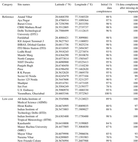
Table 1.Delhi PM sensor network sites along with the 1 h percentage data completeness with respect to the entire sampling period (i.e., from 1 January 00:00 to 31 March 2018 23:59, Indian standard time, IST; in total 90 d, 2160 h) before and after 1 h missing-data imputation for each individual site. Note that a 10 % increase in the percentage data completeness after 1 h missing-data imputation is equivalent to∼216 h of 1 h data being interpolated.
Category Site names Latitude (◦N) Longitude (◦E) Initial 1 h 1 h data completeness data after missing-data completeness imputation
Reference Anand Vihar 28.6468350 77.3160320 88 % 100 % Aya Nagar 28.4706914 77.1099364 97 % 100 % Burari Cross 28.7258390 77.2033350 98 % 100 % CRRI Mathura Road 28.5512005 77.2735737 98 % 100 % Delhi Technological 28.7500499 77.1112615 96 % 100 % University (DTU)
Faridabad 28.4088421 77.3099081 98 % 100 % IGI Airport Terminal-3 28.5627763 77.1180053 95 % 100 % IHBAS, Dilshad Garden 28.6811736 77.3025234 98 % 100 % ITO Metro Station (ITO) 28.6316945 77.2494387 98 % 100 % Lodhi Road 28.5918245 77.2273074 93 % 100 % Mandir Marg 28.6364290 77.2010670 96 % 100 % North Campus 28.6573814 77.1585447 94 % 100 % NSIT Dwarka 28.6090900 77.0325413 95 % 100 % Punjabi Bagh 28.6740450 77.1310230 94 % 100 %
Pusa 28.6396450 77.1462620 99 % 100 %
R K Puram 28.5632620 77.1869370 95 % 100 % Sector 62 Noida 28.6245479 77.3577104 93 % 99 % Sector 125 Noida 28.5447608 77.3231257 90 % 97 % Shadipur 28.6514781 77.1473105 97 % 100 % Siri Fort 28.5504249 77.2159377 78 % 100 % U.S. Embassy 28.5980970 77.1880330 95 % 100 % Vasundhara, Ghaziabad 28.6603346 77.3572563 100 % 100 %
Low-cost All India Institute of 28.5545006 77.2124023 89 % 100 % Medical Science (AIIMS)
Hiran Kudna 28.6674995 77.0089035 80 % 97 % Indian Institute of 28.5473003 77.1909027 88 % 99 % Technology Delhi (IITD)
Indian Institute of 28.6303400 77.1750400 98 % 100 % Tropical Meteorology (IITM)
Kaushambi 28.6410008 77.3199005 84 % 100 % Manav Rachna University 28.4477005 77.3084030 87 % 100 % (MRU)
Mayur Vihar 28.6079998 77.2906036 85 % 93 % Naraina Vihar 28.6289005 77.1391983 70 % 79 % New Friends Colony 28.5676994 77.2687988 99 % 100 % S.D.A. Park 28.5517006 77.2031021 66 % 97 %
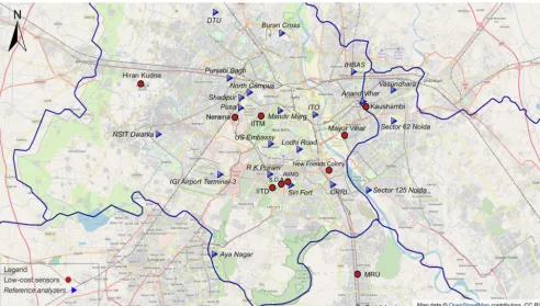
concentrations over winter season due to a combination of increased biomass burning for heating, shallower boundary layer mixing height, diminished wet scavenging by precip-itation, lower wind speed, and trapping of air pollutants by the Himalayan topology. Figure 2 visualizes the spatial dis-tribution of these 22 reference monitors (triangles with italic text) and Table 1 lists their latitudes and longitudes. No sta-tion of the 22 reference monitors is known for regional back-ground monitoring. The complex local built environment in Delhi arising from the densely and intensively mixed land
use (Tiwari, 2002) and the significant contributions to air pollution from all vehicular, industrial (small-scale indus-tries and major power plants), commercial (diesel generators and tandoors), and residential (diesel generators and biomass burning) sectors (CPCB, 2009; Gorai et al., 2018) render the PM2.5concentrations relatively unconnected to the land-use
Figure 1. (a)Front view of the low-cost node.(b)Key components of the low-cost node.
the remaining 21 Indian government monitoring stations be-cause neither the relevant Indian agencies provided QA and QC remarks or error flags in any of their regulatory moni-toring stations’ datasets nor can we obtain the QA and QC procedures (e.g., how and how often reference monitors are maintained and calibrated) for these reference monitors. Due to lack of relevant QA and QC information to exclude any measurements, all of the hourly PM2.5concentrations of the
21 monitoring stations operated by the Indian agencies were assumed to be correct. We would like to highlight this as a potential shortcoming of using the measurements from the Indian government monitoring stations. While mathemati-cally the GPR model can operate without requiring data from all the stations to be non-missing on each day by relying on only each day’s non-missing stations’ covariance infor-mation to make inference, we practically required concur-rent measurements of all the stations in this paper to drasti-cally increase the speed of the algorithm (∼10 min to run a complete 22-fold leave-one-out CV, up to∼20 times faster) by avoiding the expensive computational cost of excessive
amount of matrix inversions that can be incurred otherwise. We therefore linearly interpolated the 1 h PM2.5values for
the hours with missing measurements for each station, af-ter which we averaged the hourly data to daily resolution as the model inputs. We validate our interpolation approach in Sect. 3.2.1 by showing that the model accuracies with and without interpolation are statistically the same.
2.2.2 Low-cost node PM2.5data
Hourly uncalibrated PM2.5 measurements from 10
At-mos low-cost nodes across Delhi between 1 January and 31 March 2018 were downloaded from our low-cost sensor cloud platform. No correction or filter of any kind was ap-plied to the raw signals of the low-cost nodes over the cloud platform before we downloaded the data. Figure 2 shows the sampling locations of these 10 low-cost nodes as circles, and Table 1 specifies their latitudes and longitudes. In our cur-rent study, the factors governing the siting of these nodes consist of the ground contact personnel availability, the re-source availability such as a strong mobile network signal and 24/7 main power supply, the location’s physical acces-sibility, and some other common criteria for sensor deploy-ment (e.g., locations away from major pollution sources, sit-uated in a place where free flow of air is available, and pro-tected from vandalism and extreme weather). Similar to the pre-processing of the reference PM2.5data, we linearly
inter-polated the missing hourly PM2.5for each low-cost node and
then aggregated the hourly data at a daily interval. The com-parison of 1 h PM2.5’s completeness before and after
miss-ing data imputation for both reference and low-cost nodes is detailed in Table 1, and the periods over which data were imputed for each site are illustrated in Fig. S1 in the Sup-plement. There is no obvious pattern in the data missing-ness. To remove the prospective outliers such as erroneous surges or nadirs existing in the datasets of the 21 Indian gov-ernment reference nodes and the 10 low-cost nodes, or to remove unreasonable interpolated measurements introduced during handling the missing data, we employed the Local Outlier Factor (LOF) algorithm with 20 neighbors consid-ered (a number that works well in general) to remove a con-servative∼10 % of the 32-dimensional (22 reference+10 low-cost nodes) 24 h PM2.5 datasets. The LOF is an
5166 T. Zheng et al.: Gaussian process regression model
Figure 2.Locations of the 22 reference nodes (triangles with italic text) and 10 low-cost nodes (circles) that form the Delhi PM sensor network. ©OpenStreetMap contributors 2019. Distributed under a Creative Commons BY-SA License.
in the network were left (see Fig. S1) and used for our model evaluation.
2.3 Simultaneous GPR and simple linear regression calibration model
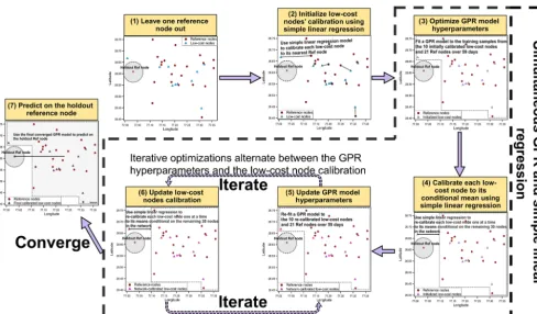
The simultaneous GPR and simple linear regression calibra-tion algorithm is introduced here as Algorithm 1. The critical steps of the algorithm are linked to sub-sections under which the respective details can be found. Complementing Algo-rithm 1, a flow diagram illustrating the algoAlgo-rithm is given in Fig. 3.
2.3.1 Leave one reference node out
Because the true calibration factors for the low-cost nodes are not known beforehand, a leave-one-out CV approach (i.e., holding one of the 22 reference nodes out of modeling each run for model predictive performance evaluation) was adopted as a surrogate to estimate our proposed model ac-curacy of calibrating the low-cost nodes. For each of the 22-fold CV, 31 node locations (denoted0= {x1, . . .,x31}) were
available, wherexiis the latitude and longitude of nodei. Let yit represent the daily PM2.5measurement of nodeion day
t andyt∈R31 denote the concatenation of the daily PM2.5
measurements recorded by the 31 nodes on day t. Given a finite number of node locations, a Gaussian process (GP)
be-comes a multivariate Gaussian distribution over the nodes in the form of the following:
yt|0∼N (µ,6) , (1)
whereµ∈R31 represents the mean function (assumed to be 0in this study);6∈R31×31 with6ij=K xi,xj;2
rep-resents the covariance function or kernel function and2is a vector of the GPR hyperparameters.
For simplicity’s sake, the kernel function was set to a squared exponential (SE) covariance term to capture the spa-tially correlated signals coupled with another component to constrain the independent noise (Rasmussen and Williams, 2006):
K xi,xj;2=σs2exp − xi−xj
2 2
2l2
!
+σn2I, (2)
whereσs2,l, andσn2 are the model hyperparameters (to be optimized) that control the signal magnitude, characteristic length scale, and noise magnitude, respectively;2∈R3is a vector of the GPR hyperparametersσs2,l, andσn2.
2.3.2 Initialize low-cost nodes’ (simple linear regression) calibrations
low-Figure 3.The flow diagram illustrating the simultaneous GPR and simple linear regression calibration algorithm. In step one, for each of the 22-fold leave-one-out CVs, one of the 22 reference nodes is held out of modeling for the model predictive performance evaluation in step seven. In step two, fit a simple linear regression model between each low-cost nodeiand its closest reference node’s PM2.5, initialize
low-cost nodei’s calibration model to this linear regression model, and calibrate the low-cost nodeiusing this model. In step three, first initialize the GPR hyperparameters to [0.1, 50, 0.01] and then update the hyperparameters based on the training samples from the 10 initially calibrated low-cost nodes and 21 reference nodes over 59 d. In step four, first compute each low-cost nodei’s means conditional on the remaining 30 nodes given the optimized GPR hyperparameters, then fit a simple linear regression model between each low-cost nodeiand its conditional means, update low-cost nodei’s calibration model to this new linear regression model, and re-calibrate the low-cost nodeiusing this new model. In steps five and six, iterative optimizations alternate between the GPR hyperparameters and the low-cost node calibrations using the approaches described in steps three and four, respectively, until the GPR hyperparameters converged. In step seven, predict the 59 d PM2.5
measurements of the holdout reference node based on the finalized GPR hyperparameters and the low-cost node calibrations.
cost nodes using a simple linear regression model into the spatial model. Linear regression has previously been shown to be effective at calibrating PM sensors (Zheng et al., 2018). Linear regression was first used to initialize low-cost nodes’ calibrations (step two in Fig. 3). In this step, each low-cost node i was linearly calibrated to its closest reference node using Eq. (3), where the calibration factorsαi (slope) andβi
(intercept) were determined by fitting a simple linear regres-sion model to all available pairs of daily PM2.5mass
concen-trations from the uncalibrated low-cost nodei(independent variable) and its closest reference node (dependent variable). This step aims to bridge disagreements between low-cost and reference node measurements, which can lead to a more con-sistent spatial interpolation and a faster convergence during the GPR model optimization.
ri=
y
i, if reference node αi·yi+βi, if low-cost node
, (3)
whereyi is either a vector of all the daily PM2.5
measure-ments of reference node i or a vector of all the daily raw PM2.5signals of low-cost nodei;ri is either a vector of all
the daily PM2.5measurements of reference nodeior a vector
of all the daily calibrated PM2.5 measurements of low-cost
node i; andαi andβi are the slope and intercept,
respec-tively, determined from the fitted simple linear regression calibration equation with daily PM2.5 mass concentrations
of the uncalibrated low-cost nodeias independent variable and PM2.5mass concentrations of low-cost nodei’s closest
reference node as dependent variable.
2.3.3 Optimize GPR model (hyperparameters)
In the next step (step three in Fig. 3), a GPR model was fit to each dayt’s 31 nodes (i.e., 10 initialized low-cost nodes and 21 reference nodes) as described in Eq. (4). Prior to the GPR model fitting, all the PM2.5 measurements of the
hy-5168 T. Zheng et al.: Gaussian process regression model
perparameters training were standardized. The standardiza-tion was performed by first concatenating all these training PM2.5 measurements (from the 31 nodes over 59 d), then
subtracting their mean µtraining and dividing them by their
standard deviationstraining(i.e., transforming all the training
PM2.5measurements to have a 0 mean and unit variance). It
is worth noting that assuming the mean functionµ∈R31to be0along with standardizing all the training PM2.5samples
in this study is one of the common modeling formulations on the GPR model and also the simplest one. More complex formulations including a station-specific mean function (lack of prior information for this project), a time-dependent mean function (computationally expensive), and a combination of both were not considered for this paper. After the standard-ization of training samples, the GPR was trained to maximize the log marginal likelihood over all 59 d using Eq. (5) and us-ing an L-BFGS-B optimizer (Byrd et al., 1994). To avoid bad local minima, several random hyperparameter initializations were tried and the initialization that resulted in the largest log marginal likelihood after optimization was chosen (in this
pa-per,2=[σs2,l,σn2]was initialized to [0.1, 50, 0.01]).
rt|0∼N (µ,6) , (4)
wheretranges from 1 (inclusive) to 59 (inclusive);rt∈R31
is a vector of all 31 nodes’ PM2.5measurements (calibrated
if low-cost nodes) on day t; 0= {x1, . . .,x31}denotes 31
nodes’ locations andxi ∈R2is a vector of the latitude and
longitude of nodei; µ∈R31 represents the mean function (assumed to be 0 in this study); and6∈R31×31with6ij= K xi,xj;2 represents the covariance function or kernel
function.
arg max 2 L (2)
=arg max 2
X59
t=1logp (rt|2) =arg max
2 (
−0.5·59·log|6θ| −0.5
X59
t=1r T t 6
−1
θ rt), (5)
2.3.4 Update low-cost nodes’ (simple linear regression) calibrations based on their conditional means Once the optimum 2 for the (initial) GPR was found, we used the learned covariance function to find the mean of each low-cost node i’s Gaussian Distribution conditional on the remaining 30 nodes within the network (i.e., µitA|B) on day t as described mathematically in Eqs. (6)–(8), and we re-peatedly did so until all 59 d ofµitA|B(i.e.,µiA|B∈R59)were found and then re-calibrated that low-cost node i based on theµiA|B. The re-calibration was done by first fitting a simple linear regression model to all 59 pairs of daily PM2.5mass
concentrations from the uncalibrated low-cost nodei(yi, in-dependent variable) and its conditional mean (µi
A|B,
depen-dent variable) and then using the updated calibration factors (slope αi and intercept βi) obtained from this newly fitted
simple linear regression calibration model to calibrate the low-cost nodeiagain (using Eq. 3). This procedure is sum-marized graphically in Fig. 3 step four and was performed iteratively for all low-cost nodes one at a time. The reasoning behind this step is given in the Supplement. A high-level in-terpretation of this step is that the target low-cost node is cal-ibrated by being weighted over the remaining nodes within the network and the6it
AB6it
−1
BB term computes the weights.
In contrast to the inverse distance weighting interpolation which will weight the nodes used for calibration equally if they are equally distant from the target node, the GPR will value sparse information more and lower the importance of redundant information (suppose all the nodes are equally dis-tant from the target node) as shown in Fig. S2.
p "
rAit ritB
#! = N
" rAit ritB #
; "
µitA µitB
# "
6itAA 6itAB 6itBA 6itBB
#!
, (6)
rAit r
it
B ∼N
µitA|B, 6Ait|B, (7)
µitA|B=µitA+6itAB6itBB−1(ritB−µitB), (8) where rAit andritB are the daily PM2.5 measurement (s) of
the low-cost node i and the remaining 30 nodes on dayt; µitA,µitB, andµitA|B are the mean (vector) of the partitioned multivariate Gaussian distribution of the low-cost nodei,the remaining 30 nodes, and the low-cost nodeiconditional on the remaining 30 nodes, respectively, on day t; and 6AAit ,
6itAB,6itBA,6itBB, and6itA|Bare the covariance between the low-cost node i and itself, the low-cost nodei and the re-maining 30 nodes, the rere-maining 30 nodes and the low-cost nodei, the remaining 30 nodes and themselves, and the low-cost nodeiconditional on the remaining 30 nodes and itself, respectively, on dayt.
2.3.5 Optimize alternately and iteratively and converge Iterative optimizations alternated between the GPR hyperpa-rameters and the low-cost node calibrations using the ap-proaches described in Sect. 2.3.3 and 2.3.4, respectively
(Fig. 3 steps five and six, respectively), until the GPR pa-rameters2converged. The convergence criteria is the differ-ences in all the GPR hyperparameters between the two adja-cent runs below 0.01 (i.e., with1σs2≤0.01, 1l≤0.01, and 1σn2≤0.01).
2.3.6 Predict on the holdout reference node and calculate accuracy metrics
The final GPR was used to predict the 59 d PM2.5
measure-ments of the holdout reference node (Fig. 3 step seven) fol-lowing the Cholesky decomposition algorithm (Rasmussen and Williams, 2006) with the standardized predictions being transformed back to the original PM2.5 measurement scale
at the end. The back transformation was done by multiply-ing the predictions by the standard deviation straining (the
standard deviation of the training PM2.5measurements) and
then adding back the meanµtraining(the mean of the training
PM2.5 measurements). Metrics including root mean square
errors (RMSE, Eq. 9) and percent errors defined as RMSE normalized by the average of the true measurements of the holdout reference node in this study (Eq. 10) were calculated for each fold and further averaged over all 22 folds to assess the accuracy and sensitivity of our simultaneous GPR and simple linear regression calibration model.
RMSE= r
1 59
yi− ˆyi
2
2, (9)
whereyi andyˆi are the true and model predicted 59 daily PM2.5measurements of the holdout reference nodei.
Percent error= RMSE
avg. holdout reference PM2.5conc.
(10)
3 Results and discussion
3.1 Spatial variation of PM2.5across Delhi
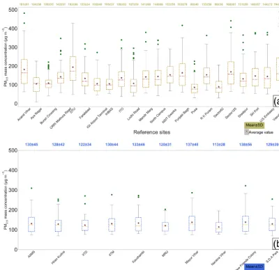
Figure 4a presents the box plot of the daily averaged PM2.5
at each available reference site across Delhi from 1 January to 31 March 2018. The Vasundhara and DTU sites were the most polluted stations with the PM2.5 averaging 194±104
and 193±90 µg m−3, respectively. The Pusa and Sector 62 sites had the lowest mean PM2.5, averaging 86±40 and
88±36 µg m−3, respectively. The Delhi-wide average of the
3-month mean PM2.5 across the 22 reference stations was
found to be 138±31 µg m−3. This pronounced spatial varia-tion in mean PM2.5in Delhi (as reflected by the high SD of
5170 T. Zheng et al.: Gaussian process regression model
Figure 4. (a)Box plots of the 24 h aggregated true ambient PM2.5mass concentrations measured by the 22 government reference monitors
across Delhi from 1 January to 31 March 2018.(b)Box plots of the low-cost node 24 h aggregated PM2.5mass concentrations calibrated by
the optimized GPR model. In both(a)and(b), mean and SD of the PM2.5mass concentrations for each individual site are superimposed on the box plots.
3.2 Assessment of GPR model performance
The optimum values of the GPR model parameters includ-ing the signal variance (σs2), the characteristic length scale (l), and the noise variance (σn2) are shown in Fig. S3. The σs2,l, andσn2from the 22-fold leave-one-out CV averaged 0.53±0.02, 97.89±5.47 km, and 0.47±0.01, respectively. The small variability in all the parameters among all the folds indicates that the model is fairly robust to the different com-binations of reference nodes. The learned length scale can be interpreted as the modeled spatial pattern of PM2.5being
relatively consistent within approximately 98 km, suggesting that the optimized model majorly captures a regional trend rather than fine-grained local variations in Delhi.
3.2.1 Accuracy of reference node prediction
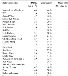
We start by showing the accuracy of model prediction on the 22 reference nodes using leave-one-out CV (when the low-cost node measurements were included in our spatial predic-tion). Without any prior knowledge of the true calibration factors for the low-cost nodes, the holdout reference node prediction accuracy is a statistically sound proxy for estimat-ing how well our technique can calibrate the low-cost nodes. The performance scores (including RMSE and percent error) for each reference station sorted by the 3-month mean PM2.5
Table 2.Summary of the GPR model 24 h performance scores (including RMSE and percent error) for predicting the measurements of the 22 holdout reference nodes across the 22-fold leave-one-out CV when the full sensor network is used. The mean of the true ambient PM2.5
mass concentrations throughout the study (from 1 January to 31 March 2018) for each individual reference node is provided. The reference nodes with the means of true PM2.5inside the range of (Delhi-wide mean±SD, i.e., 138±31) are indicated with shading.
Reference nodes RMSE Percent error Mean of true (µg m−3) PM2.5(µg m−3)
Vasundhara, Ghaziabad 68 44 % 195
DTU 56 36 % 194
Anand Vihar 47 32 % 181
Sector 125 Noida 31 23 % 169
Punjabi Bagh 26 20 % 163
NSIT Dwarka 25 19 % 153
R K Puram 26 20 % 153
Siri Fort 22 18 % 147
U.S. Embassy 21 18 % 144
North Campus 27 24 % 144
CRRI Mathura Road 27 21 % 142
Mandir Marg 16 14 % 142
ITO 15 14 % 136
Faridabad 21 18 % 133
Shadipur 23 22 % 132
Burari Cross 36 39 % 109
Lodhi Road 34 41 % 107
IGI Airport Terminal–3 29 32 % 106
Aya Nagar 34 38 % 105
IHBAS, Dilshad Garden 38 41 % 105
Sector 62 Noida 47 60 % 89
Pusa 48 70 % 86
Delhi-wide mean 33 30 % 138
SD 13 14 % 31
data because real-time reference monitors that are certified as the Federal Equivalent Methods (FEMs) by the U.S. Environ-mental Protection Agency (EPA) are required to provide re-sults comparable to the Federal Reference Methods (FRMs) only for a 24 h but not a 1 h sampling period. Our algorithm, which essentially relies on the accuracy of the reference mea-surements, can only calibrate or predict as well as the ref-erence methods measure. Therefore, only the percent error based on the reliable 24 h reference measurements is a fair representation of our algorithm’s true calibration/prediction ability. Although the technique is reasonably accurate, es-pecially considering the minimal amount of field work in-volved, its calibration error is nearly 3 times higher than the error of the low-cost nodes that were well calibrated by col-location with an environmental beta attenuation monitor (E-BAM) in our previous study (error: 11 %; RMSE: 13 µg m−3) under similar PM2.5concentrations at the same temporal
res-olution (Zheng et al., 2018). The suboptimal on-the-fly map-ping accuracy is a result of the optimized model’s ability to simulate only the regional trend well. From a different per-spective, the GPR method would have modeled the spatial pattern of PM2.5in Delhi well had the natural spatial
covari-ance among the nodes not been disturbed by the complex
and prevalent local sources there. As a substantiation of the flawed local PM2.5 variation modeling, the reference node
mapping accuracy follows a pattern, with relatively high-quality prediction for those nodes whose means were close to the Delhi-wide mean (e.g., Delhi-wide mean±SD as high-lighted with shading in Table 2) and relatively poor predic-tion for those nodes whose means differed substantially from the Delhi-wide mean (particularly on the lower end).
In this paper, we interpolated the missing 1 h PM2.5
ex-5172 T. Zheng et al.: Gaussian process regression model
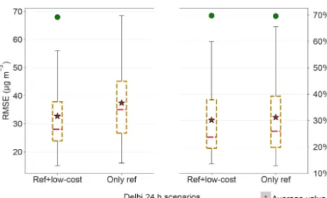
Figure 5.Box plots of the GPR model 24 h performance scores (in-cluding RMSE and percent error) for predicting the measurements of the 22 holdout reference nodes across the 22-fold leave-one-out CV under two scenarios – using the full sensor network by includ-ing both reference and low-cost nodes and usinclud-ing only the reference nodes for the model construction. Note both scenarios were given the initial parameter values and bounds that maximize the model performance.
ception of station Vasundhara whose error without interpo-lation is 10 % lower than that with interpointerpo-lation. The Delhi-wide mean percent errors with (30 %) and without interpo-lation (29 %) are also essentially the same. We further used the Wilcoxon signed-rank test (Wilcoxon, 1945) to prove that the two related paired samples (i.e., the percent errors for the 22 reference stations with and without interpolation) are in-deed statistically the same. The Wilcoxon signed-rank test is a nonparametric version of the parametric pairedttest (in-volving two related or matched samples or groups) that re-quires no specific distribution on the measurements (unlike the parametric pairedttest that assumes a normal distribu-tion). We conducted a two-sided test which has the null hy-pothesis that the percent errors for the 22 reference stations with and without interpolation are the same (i.e., H0: with =without) against the alternative that they are not the same (i.e., H1: with 6= without). Thep value of the test is 0.07.
The level of statistical significance was chosen to be 0.05, which means that the null hypothesis (i.e., H0: with=
with-out) cannot be rejected when thepvalue is 0.07 (above 0.05). Therefore, interpolating missing 1 h PM2.5data for both
ref-erence and low-cost nodes is appropriate for this paper be-cause the accuracies of model prediction on the 22 reference nodes with and without interpolation are not distinct based on the Wilcoxon signed-rank test result.
It is of particular interest to validate the value of estab-lishing a relatively dense wireless sensor network in Delhi by examining if the addition of the low-cost nodes can truly lend a performance boost to the spatial interpolation among sensor locations. We juxtapose the interpolation performance using the full sensor network (including both the reference and low-cost nodes) with that using only the reference nodes in Fig. 5. In this context, the unnormalized RMSE is less
rep-Figure 6.Box plots of the learned calibration factors (i.e., intercept and slope) for each individual low-cost node from the 22 optimized GPR models across the 22-fold leave-one-out CV.
resentative than the percent error of the model interpolation performance because of the unequal numbers of overlapping 24 h observations for all the nodes (59 data points) and for only the reference nodes (87 data points). The comparison re-vealed that the inclusion of the 10 low-cost devices on top of the regulatory grade monitors can reduce mean and median interpolation error by roughly 2 %. While only a marginal improvement with 10 low-cost nodes in the network, the out-come hints that densely deployed low-cost nodes can have great promise of significantly decreasing the amount of pure interpolation among sensor locations, therefore benefitting the spatial precision of a network. We will explore more about the significance of the low-cost nodes for the network performance in Sect. 3.3.3.
3.2.2 Accuracy of low-cost node calibration
Next we describe the technique’s accuracy of low-cost node calibration. The model-produced calibration factors are shown in Fig. 6. The intercepts and slopes for each unique low-cost device varied little among all the 22 CV folds, re-iterating the stability of the GPR model. The values of these calibration factors resemble those obtained in the previous field work, with slopes comparable to South Coast Air Qual-ity Management District’s evaluations on the Plantower PMS models (SCAQMD, 2017a–c) and intercepts comparable to our Kanpur, India post-monsoon study (Zheng et al., 2018).
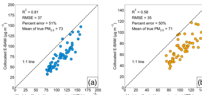
Figure 7.Correlation plots comparing the GPR model-calibrated low-cost node PM2.5mass concentrations to the collocated E-BAM
mea-surements at(a)MRU and(b)IITD sites. In both(a)and(b), correlation of determination (R2), RMSE, percent error, and mean of the true ambient PM2.5mass concentrations throughout the study (from 1 January to 31 March 2018) are superimposed on the correlation plots.
near the lower end of PM2.5spectrum in Delhi. These high
error rates echo the conditions found at the comparatively clean Pusa and Sector 62 reference sites. The scatterplots also reveal the reason why the technique especially has trou-ble calibrating low-concentration sites – the technique over-predicted the PM2.5concentrations at the low-concentration
sites to match the levels as if subject to the natural spatial variation. The washed-out local variability after model cal-ibration more obviously manifests in Fig. 4b, which stands in marked contrast to the true wide variability across the ref-erence sites (Fig. 4a). In other words, the geostatistical tech-niques can calibrate the low-cost nodes dynamically, with the important caveat that it is effective only if the degree of ur-ban homogeneity in PM2.5is high (e.g., the local
contribu-tions are as small a fraction of the regional ones as possible, or the local contributions are prevalent but of similar mag-nitudes). Otherwise, quality predictions will only apply for those nodes whose means are close to the Delhi-wide mean. Gani et al. (2019) estimated that Delhi’s local contribution to the composition-based submicron particulate matter (PM1)
was∼30 to 50 % during winter and spring months. Clearly the huge amount of local influence in Delhi did not fully sup-port our technique.
3.2.3 GPR model performance as a function of training window size
So far, the optimization of both GPR model hyperparame-ters and the linear regression calibration factors for the low-cost nodes has been carried out over the entire sampling pe-riod using all 59 available daily averaged data points. It is of critical importance to examine the effect of time history on the algorithm, by analyzing how sensitive the model per-formance is to training window size. We tracked the model performance change when an increment of 2 d of data were included in the model training. The model performance was
5174 T. Zheng et al.: Gaussian process regression model
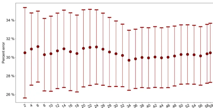
Figure 8.The mean percent error rate of GPR model prediction on the 22 reference nodes using leave-one-out CV (see Sect. 3.2.1) as a function of training window size in an increment of 2 d. The error bars represent the standard error of the mean (SEM) of the GPR prediction errors of the 22 reference nodes.
of the 22 reference nodes in that week. The performance was still measured by the mean accuracy of model prediction on the 22 reference nodes using leave-one-out CV, as described in Sect. 3.2.1. We found similarly stable 26 %–34 % dynamic calibration error rates and∼3 %–7 % SEMs throughout the weeks (see Fig. S4).
3.2.5 Relative humidity (RH) adjustment to the algorithm
We attempted RH adjustment to the algorithm by incorporat-ing an RH term in the linear regression models, where the RH values were the measurements from each corresponding low-cost sensor package’s embedded Adafruit DHT22 RH and temperature sensor. However, there was no improvement in the algorithm’s accuracy after RH correction. A plausi-ble explanation is one regarding the infrequently high RH conditions during the winter months in Delhi and stronger smoothing effects at longer averaging time intervals (i.e., 24 h). Our previous work (Zheng et al., 2018) suggested that the PMS3003 PM2.5 weights exponentially increased only
when RH was above∼70 %. The Delhi-wide average of the 3-month RH measured by the 10 low-cost sites was found to be 55±15 %. Only 17 % and 6 % of these RH values were greater than 70 % and 80 %, respectively. The infre-quently high RH conditions can cause the RH-induced biases to be insignificant. Additionally, our previous work found that even though major RH influences can be found in 1 min to 6 h PM2.5measurements, the influences significantly
di-minished in 12 h PM2.5 measurements and were barely
ob-servable in 24 h measurements. Therefore, longer averaging time intervals can smooth out the RH biases.
Additionally, while our algorithm was analyzed over the 59 available days in this study, the daily averaged temper-ature and RH measurements for the entire sampling period
(i.e., from 1 January to 31 March 2018, 90 days) were statis-tically the same as those for the 59 d. To support this state-ment, we conducted the Wilcoxon rank-sum test, also called Mann–WhitneyU test (Wilcoxon, 1945; Mann and Whit-ney, 1947) on the daily averaged temperature and RH mea-surements from the Indira Gandhi International (IGI) Air-port. The Wilcoxon rank-sum test is a nonparametric ver-sion of the parametricttest (involving two independent sam-ples or groups) that requires no specific distribution on the measurements (unlike the parametrict test that assumes a normal distribution). We did not use a paired test here be-cause the two groups had different sample sizes (i.e., 59 and 90, respectively). We conducted a two-sided test which has the null hypotheses that the daily averaged temperature and RH measurements for the 90 d (19±5◦C, 59±14 %) and the 59 d (20±5◦C, 59±12 %) were the same (i.e., H0: Temperature59 d= Temperature90 d/RH59 d = RH90 d)
against the alternatives that they were not the same (i.e., H1:
Temperature59 d6=Temperature90 d/RH59 d6=RH90 d). Thep
values for the temperature and RH comparisons are 0.28 and 0.59, respectively. The level of statistical significance was chosen to be 0.05, which means that the null hypothe-ses (i.e., H0: Temperature59 d= Temperature90 d/RH59 d=
RH90 d) cannot be rejected when thepvalues are both above
0.05. Therefore, the daily averaged temperature and RH mea-surements from the IGI Airport for the entire sampling period and for the 59 d were not statistically distinct.
3.3 Simulation results
While the exact values of the calibration factors derived from the GPR model fell short of faithfully recovering the original picture of PM2.5spatiotemporal gradients in Delhi, these
out to be useful in facilitating automated large-scale sensor network monitoring.
3.3.1 Simulation of low-cost node failure or under heavy influence of local sources
One way to simulate the conditions of low-cost node fail-ure or under heavy influence of local sources is to replace their true signals with values from random number gener-ators so that the inherent spatial correlations are corrupted. In this study, we simulated how the model-produced cali-bration factors change when all (10), nine, seven, three, and one of the low-cost nodes within the network malfunction or are subject to strong local disturbance. We have three major observations from evaluating the simulation results (Figs. 9 and S5). First, the normal calibration factors are quite dis-tinct from those of the low-cost nodes with random signals. Compared to the normal values (see Fig. 9f), the ones of the low-cost nodes with random signals have slopes close to 0 and intercepts close to the Delhi-wide mean of true PM2.5in
Delhi (most clearly shown in Fig. 9a). Second, the calibration factors of the normal low-cost nodes are not affected by the aberrant nodes within the network (see Fig. 9b,c,d,e,f). These two observations indicate that the GPR model enables auto-mated and streamlined process of instantly spotting any mal-functioning low-cost nodes (due to either hardware failure or under heavy influence of local sources) within a large-scale sensor network. Third, the performance of the GPR model seems to be rather uninfluenced by changing the true sig-nals to random numbers (see Fig. S5, 33 % error rate when all low-cost nodes are random vs. baseline 30 % error rate). One possible explanation is that the prevalent and intricate air pollution sources in Delhi have already dramatically weak-ened the natural spatial correlations. This means that a sig-nificant degree of randomness has already been imposed on the low-cost nodes in Delhi prior to our complete random-ness experiment. It is worth mentioning that flatlining is an-other commonly seen failure mode of our low-cost PM sen-sors in Delhi. The raw signals of such malfunctioning PM sensors were observed to flatline at the upper end of the sen-sor output values (typically thousands of µg m−3). The very distinct signals of these flatlining low-cost PM nodes, how-ever, make it rather easy to separate them from the rest of the nodes and filter them out at the early pre-processing stage before analyses and therefore without having to resort to our algorithm. Nevertheless, our not so accurate on-the-fly cali-bration model has created a useful algorithm for supervising large-scale sensor networks in real time as a by-product. 3.3.2 Simulation of low-cost node drift
We further investigated the feasibility of applying the GPR model to track the drift of low-cost nodes accurately over time. We simulated drift conditions by first setting random percentages of intercept and slope drift, respectively, for each
individual low-cost node and for each simulation run. Next, we adjusted the signals of each low-cost node over the en-tire study period given these randomly selected percentages using Eq. (11). Then, we rebuilt a GPR model based on these drift-adjusted signals and evaluated if the new model-generated calibration factors matched our expected predeter-mined percentage drift relative to the true (baseline) calibra-tion factors.
yi_drift= yi
(1−percentage slope drifti)
+ percentage intercept drifti ·true intercepti (1−percentage slope drifti)·true slopei
, (11) whereyi, true intercepti, true slopei, percentage intercept
drifti, percentage slope drifti, andyi_driftare a vector of the
true signals, the standard model-derived intercept, the stan-dard model-derived slope, the randomly generated percent-age of intercept drift, the randomly generated percentpercent-age of slope drift, and a vector of the drift-adjusted signals, respec-tively, over the full study period for low-cost nodei.
The performance of the model for predicting the drift was examined under a variety of scenarios including the assump-tion that all (10), eight, six, four, and two of the low-cost nodes developed various degrees of drift such as a signif-icant (11 %–99 %), a marginal (1 %–10 %), and a balanced mixture of significant and marginal. The testing results for 10, six, and two low-cost nodes are displayed in Table 3 and those for eight and four nodes are in Table S2. Over-all, the model demonstrates excellent drift predictive power with less than 4 % errors for all the simulation scenarios. The model proves to be most accurate (within 1 % error) when low-cost nodes only drifted marginally regardless of the number of nodes drift. In contrast, significant, and par-ticularly a mixture of significant and marginal drifts, might lead to marginally larger errors. We also notice that the inter-cept drifts are slightly harder to accurately capture than the slope drifts. Similar to the simulation of low-cost node fail-ure or under strong local impact as described in Sect. 3.3.1, the performance of the model for predicting the measure-ments of the 22 holdout reference nodes across the 22-fold leave-one-out CV was untouched by the drift conditions (see Fig. S6). This unaltered performance can be attributable to the fact that the drift simulations only involve simple linear transformations as shown in Eq. (11). The high-quality drift estimation has therefore presented another convincing case of how useful our original algorithm can be applied to dy-namically monitoring dense sensor networks, as a by-product of calibrating low-cost nodes.
5176 T. Zheng et al.: Gaussian process regression model
Figure 9.Learned calibration factors for each individual low-cost node from the optimized GPR models by replacing measurements of all(a), nine(b), seven(c), three(d), one(e), and zero(f)of the low-cost nodes with random integers bounded by the min and max of the true signals reported by the corresponding low-cost nodes. Note that the nine, seven, three, and one of the low-cost nodes (whose true signals are replaced with random integers) were randomly chosen.
the same as accuracy of the model trained on 2 d of data, and if the model trained on 59 d is able to detect the simu-lated drift, then so should the model trained on 2 d. Then if we reasonably assume that the drift rate remains roughly un-changed within a 2 d window, then the drift mode (linear or random), which only dictates how the drift rate jumps (usu-ally smoothly as well) between any adjacent discrete 2 d win-dows, does not matter anymore. All that matters is to track that one fixed drift rate reasonably well within those 2 d, which is virtually the same as what we already did with the entire 59 d of data.
3.3.3 Optimal number of reference nodes
Points which remain unaddressed are (1) what the optimum or minimum number of reference instruments is to sustain this technique, and (2) if the inclusion of low-cost nodes can effectively assist in lowering the technique’s calibration or mapping inaccuracy. It is interesting to note that optimizing the model’s calibration accuracy can not only directly fulfill
the fundamental calibration task, but it can also better help the sensor network monitoring capability as an added bonus. To address these two outstanding issues, we randomly sam-pled subsets of all the 22 reference nodes within the network in increments of one node (i.e., from 1 to 21 nodes) and im-plemented our algorithm with and without incorporating the low-cost nodes, before finally computing the mean percent errors in predicting all the holdout reference nodes. To get the performance scores as close to truth as possible but with-out incurring excessive computational cost in the meantime, the sampling was repeated 100 times for each subset size. The calibration error in this section was defined as the mean percent errors in predicting all the holdout reference nodes further averaged over 100 simulation runs for each subset size.
Table 3.Comparison of predetermined percentages of drift to those estimated from the GPR model for intercept and slope, respectively, for each individual low-cost node, assuming all (10), six, and two of the low-cost nodes developed various degrees of drift such as significant (11 %–99%), marginal (1 %–10 %), and a balanced mixture of significant and marginal. Note the sensors that drifted, the percentages of drift, and which sensors drifted significantly or marginally are randomly chosen. The results reported under each scenario are based on averages of 10 simulation runs.
Drift category Low-cost nodes All low-cost nodes drift Six low-cost nodes drift Two low-cost nodes drift
Intercept drift Slope drift Intercept drift Slope drift Intercept drift Slope drift
(%) (%) (%) (%) (%) (%)
True Estimated True Estimated True Estimated True Estimated True Estimated True Estimated
Significant AIIMS 58 % 57 % 54 % 54 % 74 % 71 % 46 % 47 % 0 % −1 % 0 % −1 % Hiran Kudna 43 % 30 % 50 % 52 % 66 % 61 % 53 % 53 % 62 % 64 % 45 % 44 % IITD 51 % 52 % 52 % 51 % 0 % −1 % 0 % −2 % 0 % 1 % 0 % −3 % IITM 54 % 53 % 56 % 55 % 61 % 58 % 48 % 48 % 0 % −1 % 0 % −2 % Kaushambi 61 % 62 % 73 % 72 % 70 % 70 % 49 % 48 % 0 % 0 % 0 % −2 % MRU 55 % 56 % 56 % 56 % 58 % 61 % 41 % 39 % 0 % −1 % 0 % −2 % Mayur Vihar 60 % 65 % 48 % 47 % 0 % 1 % 0 % −3 % 0 % 1 % 0 % −3 % Naraina Vihar 56 % 54 % 76 % 76 % 0 % −4 % 0 % 1 % 0 % −1 % 0 % −1 % New Friends Colony 66 % 68 % 68 % 67 % 55 % 55 % 48 % 47 % 59 % 61 % 37 % 36 % S.D.A. Park 53 % 47 % 48 % 50 % 0 % −4 % 0 % 2 % 0 % −1 % 0 % 0 %
Mean absolute difference 3 % 1 % 2 % 1 % 1 % 2 %
50 % significant AIIMS 4 % 2 % 5 % 6 % 0 % −4 % 0 % 2 % 0 % 1 % 0 % −2 % and 50 % Hiran Kudna 51 % 42 % 51 % 52 % 50 % 42 % 50 % 52 % 0 % 1 % 0 % −2 % marginal IITD 6 % 4 % 6 % 6 % 5 % 2 % 6 % 8 % 0 % 0 % 0 % −2 % IITM 56 % 52 % 40 % 40 % 64 % 58 % 47 % 48 % 0 % 1 % 0 % −3 % Kaushambi 60 % 60 % 42 % 41 % 5 % 2 % 5 % 7 % 0 % 0 % 0 % −2 % MRU 6 % 5 % 4 % 3 % 0 % −6 % 0 % 3 % 6 % 3 % 5 % 5 % Mayur Vihar 57 % 59 % 55 % 55 % 5 % 2 % 5 % 6 % 0 % 1 % 0 % −2 % Naraina Vihar 4 % 0 % 5 % 7 % 0 % −4 % 0 % 2 % 57 % 65 % 64 % 63 % New Friends Colony 6 % 5 % 6 % 5 % 0 % −3 % 0 % 2 % 0 % −1 % 0 % −1 % S.D.A. Park 53 % 48 % 61 % 61 % 59 % 58 % 64 % 64 % 0 % 0 % 0 % −1 %
Mean absolute difference 3 % 1 % 4 % 2 % 2 % 2 %
Marginal AIIMS 5 % 5 % 5 % 4 % 8 % 8 % 5 % 5 % 0 % 0 % 0 % −1 % Hiran Kudna 3 % 4 % 6 % 5 % 0 % 0 % 0 % 0 % 0 % 0 % 0 % 0 % IITD 5 % 6 % 7 % 5 % 7 % 8 % 5 % 4 % 6 % 7 % 5 % 4 % IITM 5 % 5 % 5 % 5 % 0 % 0 % 0 % −1 % 0 % 0 % 0 % −1 % Kaushambi 5 % 5 % 5 % 4 % 5 % 6 % 7 % 6 % 0 % 0 % 0 % −1 % MRU 5 % 7 % 4 % 2 % 6 % 8 % 5 % 3 % 5 % 7 % 6 % 4 % Mayur Vihar 7 % 7 % 5 % 4 % 0 % 1 % 0 % −1 % 0 % 1 % 0 % −1 % Naraina Vihar 6 % 6 % 7 % 6 % 7 % 7 % 6 % 5 % 0 % 0 % 0 % −1 % New Friends Colony 7 % 8 % 7 % 5 % 0 % 1 % 0 % −2 % 0 % 1 % 0 % −1 % S.D.A. Park 5 % 5 % 7 % 6 % 6 % 6 % 6 % 6 % 0 % 0 % 0 % −1 %
Mean absolute difference 1 % 1 % 1 % 1 % 1 % 1 %
with 1 node to ∼29 % with 21 nodes; network excluding low-cost nodes: from∼43 % to∼30 %) but are somewhat locally variable and most pronounced when five, seven, and eight reference nodes are simulated. These bumps might sim-ply be the result of five, seven, and eight reference nodes being relatively non-ideal (with regard to their neighboring numbers) for the technique, although the possibility of non-convergence due to the limited 100 simulation runs for each scenario cannot be ruled out. The 19 or 20 nodes emerge as the optimum numbers of reference nodes with the lowest er-rors of close to 28 %, while 17 to 21 nodes all yield compara-bly low inaccuracies (all below 30 %). The pattern discovered in our research shares certain similarities with Schneider et al. (2017), who studied the relationship between the accu-racy of using colocation-calibrated low-cost nodes to map urban AQ and the number of simulated low-cost nodes for their urban-scale air pollution dispersion model and
Kriging-fueled data fusion technique in Oslo, Norway. Both studies indicate that at least roughly 20 nodes are essential to start producing an acceptable degree of accuracy. Unlike Schnei-der et al. (2017), who further expanded the scope to 150 nodes by generating new synthetic stations from their es-tablished model and showed a “the more, the merrier” trend of up to 50 stations, we restricted ourselves to only realis-tic data to investigate the relationship since we suspect that stations created from our model with approximately 30 % er-rors might introduce large noise, which could misrepresent the true pattern. We agree with Schneider et al. (2017) that such relationships are location specific and cannot be blindly transferred to other study sites.
mea-5178 T. Zheng et al.: Gaussian process regression model
Figure 10.Average 24 h percent errors of the GPR model for pre-dicting the holdout reference nodes in the network as a function of the number of reference stations used for the model construction under two scenarios – using the full sensor network information by including both reference and low-cost nodes and using only the reference nodes for the model construction. Note each data point (mean value) is derived from 100 simulation runs. The error bars indicating 95 % confidence interval (CI) of the means are based on 1000 bootstrap iterations. All scenarios were given the initial pa-rameter values and bounds that maximize the model performance. Thepvalue of the Wilcoxon rank-sum test for each reference sta-tion number is superimposed, where apvalue below 0.05 means that the error when modeling with the 10 low-cost nodes is smaller than the error without them for that reference station number.
surements in comparison to modeling without them, (at least) when the number of reference stations is optimum. We did not use a paired test here because the reference nodes for algorithm training for each simulation run were randomly chosen. Specifically in our study, for each number of refer-ence stations, the two independent samples (100 replications per sample) are the 100 replications of the mean of the 24 h percent errors (in predicting all the holdout reference nodes) from the 100 repeated random simulations when modeling with and without the low-cost nodes, respectively. We con-ducted a one-sided test which has the null hypothesis that our model’s mean 24 h prediction percent errors with and without including the low-cost nodes are the same (i.e., H0:
with=without) against the alternative that the error with the low-cost nodes is smaller than the error without them (i.e.,
H1: with < without). Thepvalues of the Wilcoxon rank-sum
tests are superimposed on Fig. 10. The level of statistical sig-nificance was chosen to be 0.05, which means that the null hypothesis (i.e., H0: with=without) can be rejected in favor
of the alternative (i.e., H1: with < without) whenpvalues are
below 0.05. Figure 10 shows that the accuracy improvement when modeling with the 10 low-cost nodes is statistically sig-nificant when the optimum number of reference stations (i.e., 19 or 20) is used. Significant accuracy improvements were also observed for 17 and 18 reference stations that had com-parably low prediction errors. Therefore, we conclude that when viewing the entire sensor network in Delhi as a whole system over the entire sampling period, modeling with the 10 low-cost nodes can decrease the extent of pure interpolation among only reference stations, (at least) when the number of reference stations is optimum. The accuracy gains are still relatively minor because of the suboptimal size of the cost node network (i.e., 10). We postulate that once the low-cost node network scales up to 100s, the model constructed using the full network information can be more accurate than the one with only the information of reference nodes by con-siderable margins.
4 Conclusions
This study introduced a simultaneous GPR and simple linear regression pipeline to calibrate wireless low-cost PM sensor networks (up to any scale) on the fly in the field by cap-italizing on all available reference monitors across an area without the requirement of pre-deployment collocation cali-bration. We evaluated our method for Delhi, where 22 ref-erence and 10 low-cost nodes were available from 1 Jan-uary to 31 March 2018 (Delhi-wide average of the 3-month mean PM2.5among 22 reference stations: 138±31 µg m−3),
using a leave-one-out CV over the 22 reference nodes. We demonstrated that our approach can achieve excellent robust-ness and reasonably high accuracy, as it is underscored by the low variability in the GPR model parameters and model-produced calibration factors for low-cost nodes and by an overall 30 % prediction error (equivalent to an RMSE of 33 µg m−3) at a 24 h scale, respectively, among the 22-fold CV. We closely investigated (1) the large model calibration errors (∼50 %) at two low-cost sites (MRU and IITD with a 3-month mean PM2.5of∼72 µg m−3) where our E-BAMs
were collocated; (2) the similarly large model prediction er-rors at the comparatively clean Pusa and Sector 62 reference sites; and (3) the washed-out local variability in the model calibrated low-cost sites. These observations revealed that our technique (and more generally the geostatistical tech-niques) can calibrate the low-cost nodes dynamically, but it is effective only if the degree of urban homogeneity in PM2.5 is high. High urban homogeneity can consist of two
are prevalent but of similar magnitudes. Otherwise, quality predictions will only apply for those nodes whose means are close to the Delhi-wide mean. We showed that our al-gorithm performance is insensitive to training window size as the mean prediction error rate and the standard error of the mean (SEM) for the 22 reference stations remained con-sistent at∼30 % and∼3 %–4 % when an increment of 2 d of data were included in the model training. The markedly low requirement of our algorithm for training data enables the models to always be nearly the most updated in the field, thus realizing the algorithm’s full potential for dynamically surveilling large-scale wireless low-cost particulate matter sensor networks (WLPMSNs) by detecting malfunctioning low-cost nodes and tracking the drift with little latency. Our algorithm presented similarly stable 26 %–34 % mean pre-diction errors and ∼3 %–7 % SEMs over the sampling pe-riod when trained on the current week’s data and pre-dicting 1 week ahead, and is therefore suitable for dynamic calibration. Despite our algorithm’s non-ideal calibration ac-curacy for Delhi, it holds the promise of being adapted for automated and streamlined large-scale wireless sensor net-work monitoring and of significantly reducing the amount of manual labor involved in the surveillance and maintenance. Simulations proved our algorithm’s capability of differenti-ating malfunctioning low-cost nodes (due to either hardware failure or under heavy influence of local sources) within a network and its capability of tracking the drift of low-cost nodes accurately with less than 4 % errors for all the simula-tion scenarios. Finally, our simulasimula-tion results confirmed that the low-cost nodes are beneficial for the spatial precision of a sensor network by decreasing the extent of pure interpolation among only reference stations, highlighting the substantial significance of dense deployments of low-cost AQ devices for a new generation of AQ monitoring networks.
Two directions are possible for our future work. The first one is to expand both the longitudinal and the cross-sectional scopes of field studies and examine how well our solution works for more extensive networks in a larger geographical area over longer periods of deployment (when sensors are expected to actually drift, degrade, or malfunction). This en-ables us to validate the practical use of our method for cal-ibration and surveillance more confidently. The second is to explore the infusion of information about urban PM2.5
spa-tial patterns such as high-spaspa-tial-resolution annual average concentration basemap from air pollution dispersion models (Schneider et al., 2017) into our current algorithm to further improve the on-the-fly calibration performance by correcting for the concentration range-specific biases.
Data availability. The data are available upon request to Tongshu Zheng ([email protected]).
Supplement. The supplement related to this article is available on-line at: https://doi.org/10.5194/amt-12-5161-2019-supplement.
Author contributions. TZ, MHB, and DEC designed the study.
DEC and TZ participated in the algorithm development. TZ wrote the paper, coded the algorithm, and performed the analyses and sim-ulations. MHB and DEC provided guidance on analyses and simu-lations and assisted in writing and revising the paper. RS and SNT established, maintained, and collected data from the low-cost sen-sor network and the two E-BAM sites. TZ collected data from all the regulatory air quality monitoring stations in Delhi. RC provided funding and technical support for the project.
Competing interests. Author Ronak Sutaria is the founder of Respirer Living Sciences Pvt. Ltd, a start-up based in Mumbai, India, which is the developer of the Atmos low-cost AQ monitor. Ronak Sutaria was involved in developing and refining the hardware of Atmos and its server and dashboard, in deploying the sensors, but not involved in data analysis. Author Robert Caldow is the director of engineering at TSI and responsible for the funding and technical support but not responsible for data analysis.
Acknowledgements. The authors would like to thank CPCB,
DPCC, IMD, SPCBs, and AirNow DOS (Department of State) for providing the Delhi 1 h reference PM2.5measurements used in the current study.
Financial support. This research has been supported under the Re-search Initiative for Real-time River Water and Air Quality Monitor-ing program funded by the Department of Science and Technology, Government of India and Intel®.
Review statement. This paper was edited by Francis Pope and re-viewed by three anonymous referees.
References
Austin, E., Novosselov, I., Seto, E., and Yost, M. G.: Laboratory evaluation of the Shinyei PPD42NS low-cost particulate matter sensor, PLoS One, 10, 1–17, https://doi.org/10.1371/journal.pone.0137789, 2015.
Breunig, M. M., Kriegel, H. P., Ng, R. T., and Sander, J.: LOF: Iden-tifying Density-Based Local Outliers, available at: http://www. dbs.ifi.lmu.de/Publikationen/Papers/LOF.pdf (last access: 10 De-cember 2018), 2000.
Byrd, R. H., Lu, P., Nocedal, J., and Zhu, C.: A limited memory algorithm for bound constrained optimization, available at: http:// users.iems.northwestern.edu/~nocedal/PDFfiles/limited.pdf (last access: 10 December 2018), 1994.