End-to-End Delay Bounds for Variable Length Packet
Transmissions under Flow Transformations
Hao Wang and Jens Schmitt
DISCO Lab, University of Kaiserslautern
{wang, jschmitt}@informatik.uni-kl.de
ABSTRACT
A fundamental contribution of network calculus is the con-volution-form representation of networks which enables tight end-to-end delay bounds. Recently, this has been extended to the case where the data flow is subject to transformations on its way to the destination. Yet, the extension, based on so-called scaling elements, only applies to a setting of iden-tically sized data units, e.g., bits. In practice, of course, one often has to deal with variable-length packets. Therefore, in this paper, we address this case and propose two novel methods to derive delay bounds for variable-length packets subject to flow transformations. One is a relatively direct ex-tension of existing work and the other one represents a more detailed treatment of packetization effects. In a numerical evaluation, we show the clear superiority of the latter one and also validate the bounds by simulation results.
Categories and Subject Descriptors
C.2.m [Computer-Communication Networks]: Miscel-laneous; C.4 [Performance of Systems]: Modeling tech-niques
General Terms
Performance, TheoryKeywords
Variable length packet, demultiplexing, network calculus, packet scaling element.
1. INTRODUCTION
Network calculus has been established as a promising ap-proximative approach to queueing theory. Simply speaking, by using inequalities instead of equalities, it can circum-vent some long-standing fundamental problems in queueing theory, especially in networks with non-Poisson arrivals and multiple nodes. Network calculus was originally conceived by Cruz [5] in the early 1990s and soon after by Chang [2]. Subsequently, many researchers have contributed to it ([3,
11, 9]). The high modelling power of the network calculus has been transposed into several important applications for network engineering problems: traditionally in the Internet’s Quality of Service proposals IntServ and DiffServ, and more recently in diverse environments such as for example wire-less sensor networks [14], switched Ethernets [15], System-on-Chip (SoC) [1], or even to speed-up of simulations [10].
A key to good performance bounds is theconvolution-form expression of multi-node networks. If we describe the service provided by a node ias a lower bound process Si(s, t) for time 0≤s≤t, a tandem ofnnodes also provides a lower bound for the service process
S1⊗S2⊗ · · · ⊗Sn,
where “⊗” denotes the (min,+) convolution defined asS1⊗
S2 = inf0≤s≤t{S1(0, s) +S2(s, t)}. As a consequence, the end-to-end performance analysis can be obtained by apply-ing a sapply-ingle-node analysis. Yet, this convolution-form has a limitation: the flows in the network are assumed to be transported unaltered. However, in many real-world appli-cations a data flow is often transformed during its transfer; for instance, some parts are lost, routed to another desti-nation, or even aggregated with other data. Previous work in deterministic network calculus has proposed the so-called data scaling element [7] to model such flow transformation. A subsequent work then introduced the stochastic scaling el-ement [4], which represents the network in convolution-form and provides a flexible means of capturing actual transfor-mations. The key idea therein is to commute the scaling element with a dynamic server element recursively in or-der to obtain a single-node form representation of the net-work. However, these models have a limitation: they scale the flow only at the granularity of identical length data units (bits or packets). This is quite restrictive as many networks use variable-length packets and information and events like sending and receiving cannot be observed at the bit-level. In this paper, we therefore propose a new scaling element which respects flows as a sequence of (variable-length) pack-ets rather than just bits. The critical challenge in defining such a scaling element at the packet-level is that it should preserve the convolution-form expression of multi-node net-works. To ease the exposure we focus on an abstract but widely applicable flow transformation operation: the demul-tiplexing of packets, i.e. to thin a flow of packets by selecting only some of them, e.g. due to network operations such as routing, load balancing, or simply loss of packets.
3HUPLVVLRQWRPDNHGLJLWDORUKDUGFRSLHVRIDOORUSDUWRIWKLVZRUNIRU SHUVRQDORUFODVVURRPXVHLVJUDQWHGZLWKRXWIHHSURYLGHGWKDWFRSLHV DUHQRWPDGHRUGLVWULEXWHGIRUSURILWRUFRPPHUFLDODGYDQWDJHDQGWKDW FRSLHVEHDUWKLVQRWLFHDQGWKHIXOOFLWDWLRQRQWKHILUVWSDJH7RFRS\ RWKHUZLVHWRUHSXEOLVKWRSRVWRQVHUYHUVRUWRUHGLVWULEXWHWROLVWV UHTXLUHVSULRUVSHFLILFSHUPLVVLRQDQGRUDIHH
9$/8(722/6'HFHPEHU%UDWLVODYD6ORYDNLD &RS\ULJKWk,&67
'2,LFVWYDOXHWRROV
We are, of course not the first to treat the case of variable-length packets (though, to the best of our knowledge we are the first to take this into account under flow transforma-tions). In particular, the packetizer element [11, 3] has been introduced in network calculus to deal with flows of variable-length packets. [12, 8] have extended it to the stochastic set-tings. [12] models heavy-tailed arrivals with packet distri-butions. [8] reveals the inherent dependence brought by the packet process to the arrivals and services. We also use the packetizer but now in combination with a scaling element in order to model flow transformations at the packet level. In previous work of ours [16] we showed a novel model to under-stand the demultiplexing for first-in-first-out (FIFO) servers and to compute tighter end-to-end delay bounds. Yet, for the n-node network to preserve the convolution-form the computation of the performance measures turned out to be hard. Therefore, in this paper, we commute the packet-level scaling element and the dynamic server (as proposed for the bit level in [4]), in order to provide a tractable end-to-end delay bound computation.
The rest of this paper is organized as follows. In Section 2, we recall several fundamental definitions of network calculus and provide extensions of some of them under the assump-tion of variable length packets. In Secassump-tion 3, we present two methods to compute the end-to-end delay bounds. The first is a relatively direct extension of [4], whereas the second provides a more detailed treatment of the packetization of flows. In Section 4 we compare two methods and compare them against simulation results. We conclude in Section 5.
2. MODELLING THE DEMULTIPLEXING
OF VARIABLE LENGTH PACKET FLOWS
In this section we first recall the definitions of demultiplex-ing, the scaling element, and the packetizer. Next, we define the packet scaling element. Further, we discuss alternative system models when analyzing the end-to-end delay of a packet. Throughout the paper, the time model is discrete.In the framework of network calculus, a data flow from a source to a destination is modelled by an arrival process
A(t), which counts the number of arriving data units (bits) in time interval (0, t]. The bivariate form is accordingly
A(s, t) :=A(t)−A(s). We also denotea(t) =A(t−1, t), i.e., the arriving data units in time slott. We model the flow departing from a server as the processD(t) with the corre-sponding definition. These model the flow of bits. For many networks, the flow of bits is transformed on the way to their destination. For example, a flow can be expanded by some extra data or some parts of the flow can be lost. One in-teresting transformation is thedemultiplexing, whereby the flow is split into multiple sub-flows. For example, if a part of the original flow is routed to another destination at some node, then the flow is demultiplexed into two sub-flows, one for each destination. We denote these as two arrival pro-cessesA(1)(
t), A(2)(
t) satisfying
A(t) =A(1)(
t) +A(2)(
t),
for allt≥0. If we describe the splitting operation on the bit-level as an indicator function1{“this bit goes to destination (1)”}, which equals to 1 if term true, 0 otherwise, we have that
A(1)(
t) =Ai=1(t)1{“bitigoes to destination (1)”}. Denoting this
indicator function for biti asXi, we define the scaling
el-ement as a random process X = (Xi)i≥1 (a more general definition can be found in [4]). We denote the scaled ar-rivals asAX(t) and
AX(t) =
A(t)
i=1
Xi, ∀t≥0.
Then we can use this scaling element to model the demul-tiplexing operation. Clearly, with 1 = (1,1, . . .) we get
A(2)(
t) = A1−X(t). As we assume that the demultiplex-ing operation happens instantaneously, the scaldemultiplex-ing element has no queue.
However, in real-world the bits perhaps belong to differ-ent (variable length) packets, and transformations happen on the whole packet instead of each bit. For the demulti-plexing example, we may simply know the routing proba-bility of a complete packet to one destination. To model this (packet-level) demultiplexing operation, we need to ex-tend the scope of the scaling element. Yet, before we do that, we first integrate variable length packets into the net-work calculus framenet-work. We denote the packet lengths as a sequence of positive integer random variablesl1, l2, . . .. A packet processL(n), n≥1 is a cumulation of these r.v.’s,
L(n) =l1+l2+· · ·+ln, and ln =L(n)−L(n−1) with
L(0) = 0. A packet flow is modelled using the definition of packetizer ([3], [11]).
Definition 1 (Packetizer). Given a packet processL(n) and an arrival processA(t), anL-packetizer is a network ele-ment expressed by a functionPL(·)satisfying for allA(t), t≥
0
PL(A(t)) =L(Nt),
where
Nt= max{m:L(m)≤A(t)}. (1)
We say that a flowA(t) isL-packetized ifA(t) =PL(A(t)) for any t≥ 0. So a packet flow is anL-packetized arrival process. Note, the functionPL is not restricted to a real
network element with a queue, it can also be used to parse a bit flow (e.g., with marks) into packets and not change its timing. In the rest of this paper, we will use both meanings.
Now we consider the demultiplexing of a packet flow. We extend the definition of the scaling element.
Definition 2 (Packet Scaling Element). A packet scaling element consists of an L-packetized arrival process
A(t) =Nt
i=1li, a packet scaling processXtaking non-negative
integer values and a scaled packetized flow defined for all
t≥0as
AX(t) =
Nt
i=1
liXi.
We can use the packet scaling element to model the trans-formation of the packet flow, specifically, the demultiplexing case. liXimeansli·1{“packetigoes to destination (1)”}, i.e., de-multiplexing operates on each packet and Xi equals either
0 or 1.
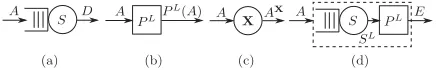
Figure 1: Network elements: (a) dynamic server, (b) packetizer, (c) packet scaling element, (d) pack-etized server.
A packet flow is usually processed or served by a queueing system before or after being demultiplexed. To analyze the delay of a packet through this system we distinguish two models. One is, after being served by each node the output is always packets, i.e., the bits are packetized by a packetizer
PL. The other is, there is no packetizer after service, yet we
observe from the bit flow the last bit of each packet accord-ing to a packet processL. In previous work [4] we derive the end-to-end delay bound for the bit flow under flow transfor-mation. The second case can be a critical challenge for that approach (L-modulated scaling process and sampling due to
L). In this paper, we focus on the first case and assume that the packetization is not changed along the path.
In network calculus, we characterize the queueing system using a dynamic server([3]). By convention, we denote it asS(s, t) for 0≤s≤t. Note that it is not the server itself but only a property of the server. It defines a lower bound process on the service such that the following convolution inequality holds for allt≥0.
D(t)≥A⊗S(t) := inf
0≤s≤t{A(s) +S(s, t)}.
When the inequality holds with equality, we say the dynamic server is exact. Note that the convolution of two concate-nated dynamic serversS1⊗S2is still a dynamic server (con-cept of convolution-form network). We define apacketized serveras a bit server followed by a packetizerPL, and
de-note the dynamic server of it asSL(s, t). Given the dynamic
server of the bit serverS and the packet processLand as-suming that a maximum packet sizelmaxexists, we obtain a possibleSL,
SL(s, t) = [S(s, t)−lmax]+. (2)
The proof follows using a busy time analysis.
We illustrate the network elements in Figure 1. Now we define the packet delay.
Definition 3 (Packet Delay). A processW(t)is called packet delay (process), if for allt≥0
W(t) = inf{d≥0 :PL(A(t))≤PL(D(t+d))}.
Here we assume the service is FIFO. The packet delay is a virtual delay that would be experienced by a packet which arrives at timet.
3. END-TO-END DELAY OF A NETWORK
WITH FLOW DEMULTIPLEXING
Figure 2: A network model consisting of packetized arrivals, services and packet scaling elements.
In this section, we compute the end-to-end packet delay for networks with multiple demultiplexers. According to previ-ous work, there are two ways to compute the end-to-end de-lay: (1) commute service and scaling elements [4], (2) get the leftover service for the flow of interest if the server uses FIFO scheduling [16]. In this paper, we use the first, i.e., we re-peatedly move all the packet scaling elements in front of the packetized servers and obtain the convolution-form of the network. Then we calculate the end-to-end delay bounds. Here, we have two choices: one is to “normalize” the packet flow as well as the bitwise service with packet size, so that the observation is directly on each packet irrespective of its size (→Section 3.1); the other is to use Definition 3 and de-rive the delay bound directly through observing the original bit flow with packetizers (→ Section 3.2). For the packet flow we assume that the packet lengths li’s are i.i.d.with
lmax<∞. In fact, this assumption can be justified in many
real-world applications with heterogeneous, large-scale, and high degree of multiplexing environment.
3.1 Observing the Packet Flow
Consider Figure 2, we lift our observation of the flow directly from the bit level to the packet level. This means we view each packet as a single data unit ignoring its size. Then we re-express the service this packet receives. After doing so we can derive the end-to-end packet delay bound directly using the calculation from [4].
Consider the arrivals consist of packets whose arrival times are defined as the arrival time of the last bit, we can model these time jumps with a counting process and together with a packet size distribution, model the arrival process as a compound process -A(t) = Ni=1(t)li, where{N(t), t ≥ 0} is the counting process, i.e., the number of arriving pack-ets in time t, andli is thei-th packet size. This seems to
be a slightly different description of a packetized flow, be-cause here we do not assume a packetizer element in the network. Yet, the packetized process resulting from pack-etizer is also covered by this definition. Consequently, we obtain an arrival process of packets -{N(t), t≥0}. We call this approach “normalization” of the bit flow by the packet sizes.
Such a sequence of packets will be served by a service ele-ment described by the bitwise service capacity together with a packetizer. How much service capacity does a packet re-ceive? To answer this question is not very hard. For exam-ple, assume that a packet with lengthlwill be served by a server with constant service capacityC bits/s, so the service rate for this packet isC/l packets/s. This is the “normal-ization” on the service side. The constant capacity server is transformed into a variable capacity server. We write it as
Snorm(s, t) =t
i=sc(i) for all 0≤s≤t. Here all thec(i)’s
are the time varying capacities of serving a packet at time
i.
In [4], we derive the end-to-end delay bounds for a flow with identically sized data units. The derivation is based on moment generating function (MGF, denoted by MX(θ) forr.v. Xand anyθ >0,MX(θ) =E[eθX]) bounds of the
arrivals and the services and expresses a network with flow transformations in a convolution-form. Therein, the servers are assumed to have constant MGF bounds. However, to use the same derivation is quite challenging, because now on one hand, the servers have variable capacities and to know their MGF bounds is hard; on the other hand, they are “normal-ized” by the same packet process and hence dependent of each other.
To obtain the MGF of the dynamic server we can firstly express the inter-service time. Then we use the (inverse) Laplace transform of the convolution of inter-arrival times and packet size distributions to compute the p.d.f.of the inter-service time. Thirdly, we use renewal theory to ob-tain the p.d.f. of the counting process of the service. At last, the MGF follows by its definition. About the depen-dency, H¨older inequality might be a solution, but many pa-rameters are introduced. We may also construct or prove some negative correlations after we use the Chernoff bound in Theorem 1 of [4]. All of these approaches lay their fo-cus on the accuracy of the expressiveness, yet, they lose the analytical tractability. In this section, we just want to pro-vide a method to calculate the end-to-end delay for variable-length packet flows that follows closely the approach in [4] and then compare it against the more sophisticated method using the packet scaling element. Assume that the bit-wise capacityS(t) is offered work-conserving with variant rates and let S(t) ≥ Ct for anyt ≥ 0 such that MGF bound
MS(t)(−θ) ≤ e−θCt for θ > 0, then we can vaguely write
c(i) ≥C/lx, where lx means either some packet length or ∞. We assume the packet size has a limit, i.e., lx≤lmax.
Clearly, c(i) ≥ C/lmax. We obtain a lower bound of this normalized dynamic serverSnorm(s, t)≥ C
lmax(t−s). Now, we represent the dynamic server as a server with the nor-malized capacity -C/lmax. And this solves the above
prob-lems at the same time. Consider the same network sce-nario as in Theorem 1. We assume the compound process as the arrivals instead of using packetizer. We also assume
MSj(t)(−θ)≤e
−θCjt, j≥1 at each bit server. The end-to-end delay has the following stochastic bound
P r(W > d)≤Knbd .
We point out, the only difference between this result and Theorem 1 in [4] is that the MGF bound of each service is
MSnorm
i (s,t)(−θ)≤e
−θlmaxCi (t−s)
. (3)
We also point out, when we do the “normalization” to the service, whether there exists a real packetizer component or not does not change the packet delay analysis, because only after the last bit of a packet is served by the bit-wise server, the service of this packet is considered to be finished, this is just as if there was a packetizer virtually.
3.2 Observing the Original Bit Flow with
Pack-etizers
In the previous subsection, we provided an approach to cal-culate end-to-end delay bounds for variable-lengths packet flows under flow demultiplexing which observes a flow on
Figure 3: Commutation of packetized service and packet scaling.
the packet-level rather than the bit level. Now we directly observe the flow on the bit level as in Figure 2. From [4] we know when deriving the end-to-end delay bound we should avoid summing up the delay bounds node-by-node, but rather use the “pay burst only once” principle. To do so, we express the network in convolution-form through moving the scaling elements between two servers to the front. The challenge now is that the scaling element is not at the bit level anymore. We provide the following lemma to commute the service and scaling element at packet-level, which is in-strumental to the derivation of end-to-end delay bounds.
Lemma 1. (Commutation of Packet Scaling
Ele-ment and Dynamic Server). Consider system (a) and (b) with packetized arrivals A(t) =PL(A(t)) in Figure 3. We defineTL(s, t) :=Nt
i=Ms+1liXias the exact dynamic server in (b), where A(s) =Ms
i=1li,A(s) +SL(s, t) =
Nt
i=1li. If
A,S,X, andLare independent, then for allt≥0,
F(t)≤EX(t).
The proof follows by using the definitions of the exact dy-namic server and TL. See details in [17]. Through this lemma, we see that there are less departures for the trans-formed system than in the original system, which ensures that the delays are higher. The expression ofTLlooks
com-plicated, but the meaning is clear. Nt
i=Ms+1liare the pa-ckets served from time s tot. And because after passing through a scaling element X, only a scaled part of these packets is sent to the next server, the service they received should also be a scaled part of the total service. After re-cursively using this lemma we get an expression for the net-work in terms of a scaled arrival process served by a dynamic server in convolution-form. The arrivals have the form
⎛ ⎜
⎝· · ·AX1X2 . ..
⎞ ⎟ ⎠
Xk
(t),
if there are k packet scaling elements. We denote it as
A(k)(
t). The alert reader may note that, for the bit flow, the concatenation of scaling elements can be naturally
for-mulated as AX1X2(
t) = A(t)
j=1X1,j
i=1 X2,i, whereas for
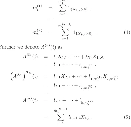
the packet flow, this is not true any more. We point out that they are just different in appearance but the same in essence - after each round of scaling we choose a part of the packets (bits) from the input flow. Therefore, we pro-vide the delicate expression of A(k)(t), which will be used in the rest of this section. Assume an L-packetized flow
A(t) =l1+l2+· · ·+lNt, whereNtis given in Eq. (1). We first denote the packets respectively the number of packets in the arrivals until timetafter each round of scaling aslk,i respectivelym(tk). Clearly fork >0
m(0)t = Nt,
m(1)t = m(0)t
i=1 1{X1
,i>0} ,
· · ·
m(tk) = m(tk−1)
i=1 1{X
k,i>0} . (4)
Further we denoteA(k)(
t) as
AX1(t) = l
1X1,1+· · ·+lNtX1,Nt = l1,1+· · ·+l
1,m(1)t ,
AX1X2(t) = l
1,1X2,1+· · ·+l1,m(1) t X2,m(1)t = l2,1+· · ·+l2,m(2)
t ,
· · ·
A(k)(t) = lk,1+· · ·+lk,m(k) t
=
m(tk−1)
i=1
lk−1,iXk,i. (5)
Next, we provide two useful lemmas for deriving the end-to-end delay bounds. The proofs can also be found in [17].
Lemma 2 (Stationarity Bound). Assume that the pa-ckets li’s of a packet process L are i.i.d. , the Xi’s of a packet scaling elementX are also i.i.d. ,AandBare two
L-packetized arrival processes, then for alls, t, x >0,
P r
AX(t)−BX(s)≥x
≤P r
(A(t)−B(s))X≥x
.
Lemma 3. (Recursive MGF Bound of Scaled
Pro-cess). Assume thatAis anL-packetized process, SLi is the packetized server,li’s are i.i.d. with maximal lengthlmax<
∞, and Xi’s are Markov-Modulated On-Off (MMOO) loss
processes and independent ofAandSLi, if we denoteVn−1(θn)
as
E
eθ
···(A(t−s)−SL1(s,u1))X1−···−Sn−L 1(un−2,un−1)Xn−1
,
then for all0≤s≤u1≤ · · · ≤un−1≤t, andn >1,
Vn−1(θn)≤e−θn−1S
L
n−1(un−2,un−1)
Vn−2(θn−1), whereθi>0,1≤i≤nis given in the proof.
We now derive the end-to-end delay bound and show that it grows inO(n) wherenis the number of nodes.
Theorem 1. (End-to-end Delay Bounds in a Packet
Flow Transformation Network). Consider the network scenario from Figure 2 where anL-packetized arrival process
A(t) =PL(A(t))traverses a series of stationary and
(mu-tually) independent bit level service elements followed by an
L-packetizer and scaling elements denoted bySL
1, SL2, . . . , SnL
and i.i.d. loss processesX1, X2, . . . , Xn−1, respectively. As-sume the packet lengths ofL-li’s are i.i.d. . Assume the
MGF bounds MA(s,t)(θ) ≤ eθrA(θ)(t−s) and MSk(t)(−θ) ≤
e−θCkt, for k = 1,2, . . . , n, and some θ > 0. We also
assume that the maximum packet length lmax < ∞.
Un-der a stability condition, to be explicitly given in the proof, forθi>0, i= 1,2, . . . , n, we have the following end-to-end steady state delay bounds for alld≥0
P r(W > d)≤e( n
i=1θi+θ1)lmaxKn
bd, (6) where the constants K and b are also given in the proof. Moreover, theε-quantiles scale asO(n), forε >0.
Proof. First we use Lemma 1 to transform the system view. To do so, we iteratively commute the packetized server and the packet scaling elementktimes. See Figure 4. Since the output of the transformed system is smaller than or equal to the original system, the delay bound of the trans-formed one must be larger than or equal to the delay bound of the original one, hence, we compute the delay bound of this transformed system.
Figure 4: Apply Lemma 1 forktimes.
Next, fixt, d≥0. Fork, s≥0 we defineU0(s, u0) =A(s), foru0=s, and then recursively
Uk(s, uk) =
Uk−1(s, uk−1) +SkL(uk−1, uk)
Xk
fork≥1 anduk−1≤uk. We prove the theorem at the first
steps by induction. Fork≥1 we assume the following two statements (S1) and (S2) for the induction:
(S1) P r(Wk(t)> d)≤ 0≤s≤t
s≤u1≤···≤uk−1≤t+d
P r
A(k−1)(t)> Uk−1(s, uk−1) +SkL(uk−1, t+d)
,
and for fixedsanduk,
(S2)
A(k−1)(s) +TkL−1⊗SLk(s, uk)
Xk
= inf
s≤u1≤···≤ukU
k(s, uk),
whereTL
k is defined recursively asT0L(0) = 0,T0L(s) =∞ for alls >0, and forNsthe number of packets inA(s)
TkL(s, uk) := Nuk
i=m(sk−1)
lk−1,iXk,i,
where
m(sk−1)
i=1
lk−1,i=A(k−1)(s),
Nuk
i=1
lk−1,i=A(k−1)(s) +TkL−1⊗SkL(s, uk). (7)
First we prove the initial step of the induction, i.e.,k= 1. For statement (S1), we have
P r(W1(t)> d) = P r(A(t)> D(t+d))
≤ P r
A(t)> A⊗S1L(t+d)
≤
0≤s≤t
P rA(t)> A(s) +SL1(s, t+d)
= 0≤s≤t
P r
A(0)(t)> U0(s, u0) +SL1(s, t+d)
.
In the first line we used the definition of packet delay. In the second line we used the definition of dynamic server. And in the third line we expanded the convolution and used Boole’s inequality. In turn for statement (S2), we have
A(0)(s) +T0L⊗S1L(s, u1)
X1
=
A(s) + inf
s≤x≤u1
T0L(s, x) +S1L(x, u1)
X1
=
A(s) +S1L(s, u1)
X1
= inf
s≤u1
A(s) +S1L(s, u1)
X1
= inf
s≤u1
U0(s, u0) +S1L(u0, u1)
X1
= inf
s≤u1U1 (s, u1).
In the third line we used thatTL
0(0) = 0, T0L(s) =∞. In the fourth line we rewrote the third line using inf, becausesand
u1are actually fixed. In the fifth line we used the definition ofU0. In the last line we used the recursive definition ofUk.
For the induction we next assume that (S1) and (S2) hold for
k≥1. Then we prove them fork+ 1. Using the argument from the initial step of the induction we can write the end-to-end delay until thek+ 1thnode
P r(Wk+1(t)> d)
≤ P r
A(k)(t)≥ inf 0≤s≤t+d
A(k)(s) +TkL⊗SkL+1(s, t+d)
≤
0≤s≤t
s≤uk≤t+d
P rA(k)(t)≥A(k)(s) +TkL(s, uk)
+SLk+1(uk, t+d)
=
0≤s≤t
s≤uk≤t+d
P r
A(k)(t)≥
m(sk−1)
i=1
lk−1,iXk,i+
Nuk
i=m(sk−1)
lk−1,iXk,i+SkL+1(uk, t+d)
=
0≤s≤t
s≤uk≤t+d
P r
A(k)(t)≥
Nuk
i=1
lk−1,iXk,i+
SkL+1(uk, t+d)
=
0≤s≤t
s≤uk≤t+d
P r
A(k)(t)≥A(k−1)(s) +
TkL−1⊗SLk(s, uk)
Xk+SL
k+1(uk, t+d)
=
0≤s≤t
s≤uk≤t+d
P rA(k)(
t)≥ inf
s≤u1≤···≤uk
Uk(s, uk)
+SLk+1(uk, t+d)
≤
0≤s≤t
s≤u1≤···≤uk≤t+d
P rA(k)(t)≥Uk(s, uk) +
SLk+1(uk, t+d)
.
In the third line we expanded the convolution and used Boole’s inequality. In the fourth line we used Eq. (4), (5), and (7). In the sixth line we used Eq. (7) again. Next we used the inductive hypothesis for (S2) and Boole’s inequal-ity in the last two lines, which completes the induction for (S1).
To prove (S2) fork+ 1 we have
A(k)(s) +TkL⊗SLk+1(s, uk+1)
X
k+1
=
A(k)(s) + inf
s≤uk≤uk+1
TkL(s, uk) +SkL+1(uk, uk+1)
Xk+1
= inf
s≤uk≤uk+1
A(k)(s) +TkL(s, uk) +SLk+1(uk, uk+1)
Xk+1
= inf
s≤uk≤uk+1
m(k−1) s
i=1
lk−1,iXk,i+ Nuk
i=m(sk−1)
lk−1,iXk,i
+SLk+1(uk, uk+1)
Xk+1
= inf
s≤uk≤uk+1
⎛ ⎝
Nuk
i=1
lk−1,iXk,i+SLk+1(uk, uk+1)
⎞ ⎠
Xk+1
= inf
s≤uk≤uk+1 A (k−1)(
s) +TkL−1⊗SkL(s, uk)Xk
+SLk+1(uk, uk+1)
Xk+1
= inf
s≤uk≤uk+1
inf
s≤u1≤···≤ukU
k(s, uk) +SkL+1(uk, uk+1)
Xk+1
= inf
s≤u1≤···≤uk+1Uk+1
(s, uk+1).
In the sixth line we used Eq. (7). In the seventh line we used the induction hypothesis. In the last line we used the definition ofUk.
Next, we use the statement (S1) to compute the end-to-end delay bound onWn(t) fork=n. We have
P r(Wn(t)> d)
≤
0≤s≤t
s≤u1≤···≤un−1≤t+d
P r
A(n−1)(t)>
· · ·
(A(s) +SL1(s, u1))X1+SL2(u1, u2)
X2+· · ·
+SnL−1(un−2, un−1)
Xn−1
+SLn(un−1, t+d)
≤
0≤s≤t
s≤u1≤···≤un−1≤t+d
P r
· · ·(A(t−s)−
S1L(s, u1))X1−SL2(u1, u2)
X2− · · · −
SnL−1(un−2, un−1)
Xn−1
> SLn(un−1, t+d)
≤
0≤s≤t
s≤u1≤···≤un−1≤t+d
e−θnSLn(un−1,t+d)·
E
e
θn
···(A(t−s)−S1L(s,u1))X1−SL2(u1,u2)X2−
···−Sn−L 1(un−2,un−1)
Xn−1
≤
0≤s≤t
s≤u1≤···≤un−1≤t+d
e−θnSLn(un−1,t+d)
e−θn−1SLn−1(un−2,un−1)· · ·
e−θ1SL1(s,u1)
eθ1rA(θ1)(s,t)
.
In the second line we expanded the recursion in the state-ment (S1). In the third line we repeatedly applied the sta-tionarity bound from Lemma 2. In the fourth line we used Chernoff’s Bound for someθn >0. In the fifth line we
re-cursively applied Lemma 3. To do so, we letθiRi−1(θi) =
logMl(θi−1), which is already stated in Lemma 3,Ri−1(θi) =
1
θilogMXi−1(logMl(θi)). Here, allS
L
i’s are packetized
dy-namic servers in the form of Eq. (2). Note that, if we let
b= sup
e−θnCn, e−θn−1Cn−1, . . . , e−θ1C1 , (8) we have
P r(Wn(t)> d)
≤
0≤s≤t
ed·logbeni=1θilmaxe(logb+θ1rA(θ1))(t−s)
·
s≤u1≤···≤un−1≤t+d
1
≤ bdeni=1θilmaxKn
.
Here we letK= (1+dn) 1+d
n
(d n)
d n
and used logb+θ1rA(θ1)<0
as the stability condition. Takingt→ ∞proves the result. We used the same argument as in [6] for the last step of computation. Finally, the order of growth of theε-quantiles for 0< ε <1 follows directly asO(n).
4. NUMERICAL EVALUATION
To evaluate the analytical results, we use the following nu-merical example settings. First, we let the packet sizes be discrete uniformly distributed i.i.d. r.v.’s, l ∼ U[a, b]. Thus, we know Ml(θ) = e
aθ−e(b+1)θ
(b−a+1)(1−eθ). Leta= 1, b= 16 for illustration. Clearly, lmax = 16. Next, we use the
Bernoulli process as the scaling process -X∼B(p), where
prepresents the data through probability, so that we know
R(θ) = 1
θlog(1−p+pMl(θ)). Further we assume that all
servers are work-conserving with constant bit rateCi. Next,
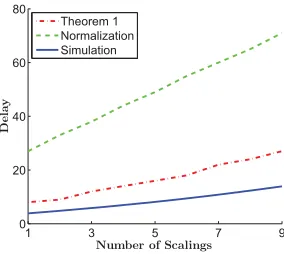
we first compare the delay bounds from Section 3.1 with those from Section 3.2 (→ Theorem 1) and also validate them against simulation results. Then we evaluate our main result from Theorem 1 changing the scaling parameters.
For the first comparison we assume that the arrivals are a compound process instead of being packetized by a packe-tizer before being served. Note, our results in Theorem 1 also imply this case, since the MGF bound of the arrival process that the theorem requires can be given directly. Without loss of applicability in real-world, we assumeA(t) is a com-pound Poisson process, so thatrA(θ) =1
θλ(Ml(θ)−1). The
average rate of the Poisson processN(t) is normalized to one
1 3 5 7 9
0 20 40 60 80
Number of Scalings
De
la
y
Theorem 1 Normalization Simulation
Figure 5: Delay bounds with Theorem 1, “normal-ized” flow, and simulation.
data unit (bit) per one time unit, i.e.,λ= 1. The number of the scaling elements varies from 1 to 9, which means maxi-mal 10 servers. We assume the utilization of the first server is 0.8, so C1 = 1.25. To choose C2, . . . , C10, we refer to Eq. (8). Avoiding that some server becomes the bottleneck, we can let all the terms in Eq. (8) be equal, i.e., θiCi =
θi−1Ci−1,2 ≤ i ≤n, where θi’s are implied in Lemma 3.
This is actually a criterion to assign the service capacities along the path a flow traverses. It must not be so strict, or in other words, the service capacities in practice may already be set before we know the other network settings. So here, for simplicity, we just statically set the capacities as
C2. . . C10= [1.15,1.05,0.95,0.85,0.80,0.75,0.70,0.65,0.60]. The quantileεis set to 10−3. We use Omnet++ to do the simulations. We measure 106 packet delays at the destina-tion node and use the empirical quantile from these for the simulation results. This will increase the result accuracy so that we ignore the confidence intervals.
Figure 5 shows the bounds on the 10−3-quantiles of the de-lay. The plot shows theO(n) order of growth. We observe that the results from Theorem 1 are much closer to the simu-lation results than the results from analyzing the normalized flow. The mathematical reason is that, although with both methods we used the maximum packet size lmax, in
The-orem 1 we used the form of [Ci·t−lmax]+, while for the normalization we used the form of Ci/lmax·t. Obviously, the loss in precision caused by the division is higher than for subtraction. The gap to the simulation results implies that the tightness still can be improved. Yet, as this work is the first attempt to model the variable length packet flow transformation, we focused on the expression of such a net-work scenario and provided the first insights calculate delay bounds in this setting. The key to improve on the tightness will be to make smarter usage of the packet length distribu-tion, than just resorting tolmax. On the other hand, as you
can also see in [11, 3], it can circumvent several technical difficulties, otherwise we would have to consider the inher-ent correlations among arrivals, services and packet scaling elements, which is, however, as we discussed in previous sec-tions or in [12, 8], very difficult even in the single node case without flow transformations. Furthermore, the usage of Boole’s inequality could be improved by the construction of a martingale as in [13]. Yet, again this is, so far only possible for the single node case. So, we leave this for future work.
1 3 5 7 9 0
100 200 300 400 500
Number of Scalings
De
la
y
Theorem 1 (p=0.3) Simulation (p=0.3) Theorem 1 (p=0.75) Simulation (p=0.75)
Figure 6: Delay bounds with Theorem 1 and the simulation.
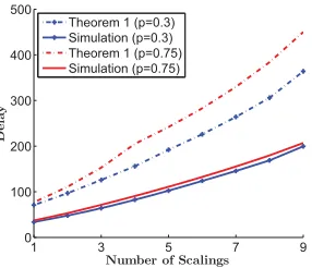
For the second comparison we slightly change the arrival de-scription. Frequently we only know the statistical properties of the bit flow and that the bits are packetized. The result from Theorem 1 can also deal with this. So we use a bit flow followed by a packetizer as the arrival for the server. Assume that the original arrival flow of bits is a Poisson process
P oi(λ). Then we knowrA(θ)(s, t)≤ λ(e
θ−1)
θ (t−s) +lmax.
The other numerical settings we use the same as before.
Figure 6 shows the bounds on the 10−3-quantiles of the delay under varying scaling parameters. We can see that Theo-rem 1 increases with the through probabilityp. That means if more of the flow is kept during the transformation, the higher the burstiness at the next server node will become. Interestingly, the gap between those curves from the theo-rem is larger than that of the simulation results. The reason is that we uselmax/C as the extra latency for each packet after being served by the packetized server, while actually most packets have a much smaller latency increase. This treatment enlarges the sensitivity of the results, because the more the flow passes through, the more tightness we lose.
5. CONCLUSION
In this paper, we extended network calculus to model net-works with variable length packet flow transformations. The main contribution is the definition of a scaling element that works on the packet level (rather than the bit level). This facilitates a commutation of the service element with the scaling element on the packet level, and thus preserves the convolution-form expression of this kind of networks. Based on this we derived the end-to-end delay bounds. We also discussed another method, which is a direct extension of a previous model by normalizing the bit flow and the bit-wise service with the packet sizes, as if the flow was treated as a flow with identical data units and the service rate was in
packets/s. We evaluated both methods and validated them against simulations. We found that the method based on the new packet scaling element is much closer to the simulation results than the other one. However, we also point out that improving the tightness is still a challenge for future work. We hope to achieve this by finding a more precise expression for the dynamic server of the packetized service.
6. REFERENCES
[1] S. Chakraborty, S. Kuenzli, L. Thiele, A. Herkersdorf, and P. Sagmeister. Performance evaluation of network processor architectures: Combining simulation with analytical estimation.Computer Networks, 42(5):641–665, April 2003.
[2] C.-S. Chang. Stability, queue length and delay of deterministic and stochastic queueing networks.IEEE Transactions on Automatic Control, 39(5):913–931, May 1994.
[3] C.-S. Chang.Performance Guarantees in Communication Networks. Springer-Verlag, 2000. [4] F. Ciucu, J. Schmitt, and H. Wang. On expressing
networks with flow transformation in
convolution-form. InProceedings of IEEE INFOCOM, pages 1979–1987, April 2011.
[5] R. L. Cruz. A calculus for network delay, Part I and II.IEEE Transactions on Information Theory, 37(1):114–141, January 1991.
[6] M. Fidler. An end-to-end probabilistic network calculus with moment generating functions. In Proceedings of IEEE IWQoS, pages 261–270, June 2006.
[7] M. Fidler and J. Schmitt. On the way to a distributed systems calculus: An end-to-end network calculus with data scaling. InProceedings of ACM
SIGMETRICS/Performance, pages 287–298, 2006. [8] Y. Jiang. Stochastic service curve and delay bound analysis: A single node case. InProceedings of the 25th International Teletraffic Congress (ITC 25), September 2013.
[9] Y. Jiang and Y. Liu.Stochastic Network Calculus. Springer-Verlag, 2008.
[10] H. Kim and J. C. Hou. Network calculus based simulation: theorems, implementation, and evaluation. InProceedings of IEEE INFOCOM, March 2004. [11] J.-Y. Le Boudec and P. Thiran.Network Calculus A
Theory of Deterministic Queuing Systems for the Internet. Number 2050 in Lecture Notes in Computer Science. Springer-Verlag, 2001.
[12] J. Liebeherr, A. Burchard, and F. Ciucu. Delay bounds in communication networks with heavy-tailed and self-similar traffic.IEEE Transactions on Information Theory, 58(2):1010–1024, February 2012. [13] F. Poloczek and F. Ciucu. Scheduling analysis with
martingales.Performance Evaluation, 79:56–72, September 2014.
[14] J. Schmitt and U. Roedig. Sensor network calculus - a framework for worst case analysis. InProceedings of IEEE DCOSS, pages 141–154, June 2005.
[15] T. Skeie, S. Johannessen, and O. Holmeide. Timeliness of real-time IP communication in switched industrial ethernet networks.IEEE Transactions on Industrial Informatics, 2(1):25–39, February 2006.
[16] H. Wang, F. Ciucu, and J. Schmitt. A leftover service curve approach to analyze demultiplexing in queueing networks. InProceedings of VALUETOOLS, pages 168–177, October 2012.
[17] H. Wang and J. Schmitt. Delay bounds calculus for variable length packet transmissions under flow transformations. Technical Report 390/14, University of Kaiserslautern, Germany, November 2014.