Energy Vector and Time Vector in the Dirac
Theory
Christian Rakotonirina
∗Institut Sup´erieur de Technologie d’Antananarivo, IST-T†
Laboratory of Dynamic of the atmosphere, of the Climate and of the Oceans, Dyaco, Antananarivo University
Madagascar
August 4, 2020
Abstract
We have introduced a sign operator of energy, analogous to the oper-ator helicity, but in the direction of what we call energy vector. How-ever, this energy vector need time vector. For giving physical senses to the components of such time vector we try to explain the time di-lation in special relativity in terms of them and try to relate them to the tunnelling times when an electron crosses a potential barrier.
Keywords : Tunnelling time, helicity, time dilation, Dirac equation, super-luminal velocity.
Introduction
Mysteries of time incresease as physics penetrate deeper and deeper into na-ture’s secrets. [1] said ”The treatment of time in quantum mechanics is one of the important and challenging open questions in the foundations of quantum theory”.
The title of the paper make us think immediately to three dimensional time. Three dimensional time theories are not something news. Many literatures have already spoken about them. Among other are [2–6]. At our side we
∗[email protected], https://orcid.org/0000-0003-0123-4813
have been by chance fallen to this question when we have encountered what we call energy vector. But, many different time quantities : tunnelling times, decay times, dwell times, delay times, arrival times, or jump times in quan-tum mechanics and proper time, time dilation in special relativity make us dare to introduce time vector in the Dirac theory, a quantum relativistic the-ory which put time and space on an equal footing.
The resolution of the Dirac equation by using the tensor product or Kro-necker product of matrices gives rise an operator [7] whose eigenvalues are the negative energy and the positive energy. We called this operator the ”sign operator of energy”. Both this operator and the operator helicity are vectors in the Pauli algebra. Their components with respect to the Pauli basis (σ1, σ2, σ3) are, respectively the components of what we call energy
vector and the momentum vector. We know that the phase of a wave func-tion solufunc-tion of the Dirac equafunc-tion is a combinafunc-tion of the components of the momentum vector coupled to the components of the position vector, that is the scalar product ~p.~x, and the energy coupled with the classical time, that is Et. So, if we consider the energy vector, time vector should be needed in the phase of the wave function. However, we should give senses to the com-ponents of this time vector, in order to know in what situations we should consider them.
We will study at first the time vector for a free electron and will try to explain the time dilation in special relativity.
The components of a time vector and any combinations of these com-ponents would evolve simultaneously from the begining to the ending of a phenomenon like the passage time and the dwell time in quantum tunnelling, from the entrance to the outrance of a potential barrier. So it is normal to think that we will able to give senses to the components of the time vector by using the tunnelling times in quantum tunnelling.
Our method consist to put forward some hypotheses for the couplings of energies with different combinations of the components of the time vector, for example the magnitude of the energy vector couples with magnitude of the time vector, and try to find out what combinations of the components of the time vector couples with the same energy as couples with such and such tunnelling time. It follows what combination of components of the time vector is equal to the tunneling time.
1
Sign Operator of energy in the Dirac
The-ory
The Dirac equation [8]
i~γµ∂µψ−mcψ = 0 (1)
is the quantum relativistic equation for a free spin-12 fermion, where the γµ’s are the gamma matrices. In this equation ~ is the Planck constant, c the speed of light, m the mass of the spin-12 fermion and ψ is its wave function. Throughout this paper we use the Dirac representation, where the gamma matrices are
γ0 =σ3⊗σ0, γ1 =iσ2⊗σ1, γ2 =iσ2⊗σ2 γ3 =iσ2⊗σ3
with
σ1 =
0 1 1 0
, σ2 =
0 −i
i 0
, σ3 =
1 0 0 −1
and σ0 =
1 0 0 1
are the Pauli matrices and σ0 the 2×2-unit matrix.
The wave function solution of the Dirac equation may be written as Kronecker product or tensor product (See, for instance [9])
ψ(t, ~x) =ξ⊗se−~i(±Et−~p.~x) (2)
of the energy stateξe−i~(±Et−~p.~x)and helicity states, whereξ=|ξ(E, p)i=
q E+mc2
2E
1
cp E+mc2
is the eigenvector associated to the positive energy E =
+pc2p2+m2c4 orξ =
ξ¯(E, p)
=
q E+mc2
2E
−E+cpmc2
1
, eigenvector
associ-ated to the negative energy −E =−pc2p2+m2c4 of the hamiltonian
oper-ator hD = cpσ1 +mc2σ3, and s is the eigenvector of the helicity operator
~
2~σ.~n, that is the spin operator in the direction of the momentum vector
~ p= p1 p2 p3
, with~n= ~ p
k~pk =
~ p p = n1 n2 n3 .
In all of that is the sign of the helicity or the handedness.
We called the operator hD =cpσ1+mc2σ3 ”sign operator of energy” [7, 10].
Let us introduce the ”energy vector” E~ =
cp 0 mc2
. Therefore, the operator
~ 2 hD E = ~ 2 ~ σ. ~E
energy vector E~. Let us call the eigenvalues of this operator ”enginity” and this operator the ”enginity operator”. Therefore there is the probabilities of the particle of having the positive enginity +~
2 or the negative enginity −~2.
For seeing that more clearly let us compare the enginity operator with the helicity operator.
hD =cpσ1+mc2σ3 hamiltonian operator ~σ.~p=p1σ1+p2σ2+p3σ3
letE~ =
cp 0 mc2
energy vector with ~p= p1 p2 p3
momentum vector
E = ~ E = p
m2c4+c2p2 the energy p=k~pk=pp2
1+p22+p23
~
2EhD =
~
2Ecpσ
1+ ~
2Emc
2σ3 ~
2p~σ.~p=
~
2pp1σ1+
~
2pp2σ2+
~
2pp3σ3
enginity operator helicity operator or spin operator in the direction ofE~ spin operator in the direction ofp~ hD
E =
cp E σ
1+ mc2
E σ
3 enginity sign ~σ.~p
p =
p1
pσ1+ p2
p σ2+ p3
p σ3 helicity
operator sign operator
Probability for having positive Probability for having positive or negative enginity (energy) or negative helicity So, a spin-12 particle can be in a superposition of a state of positive and
a state of negative energy.
But, as we have said in the introduction, energy vector E~ =
cp 0 mc2 need
time vector~t=
t1 t2 t3 .
2
Components of the Time Vector
Let us at first regard an electron with mass m, moving freely along anxaxis, from a point O to a point A of this axis. An observer observes the motion of the electron in a frame where the electron is at rest. So, this observer can mesure the time, the proper time τ =t3 that takes the electron for moving
fromO toA. For calculating the energy of the electron this observer use the formula E =mc2.
Now let us see how an observer in a frame fixed at the point O, mesures the time that takes the electron for moving from O toAwith velocity v and how he calculates the energy of the electron. For this observer, Ais at a distance
L fromO. The electron takes the impulsion p= √ mv
1−(v/c)2, and the observer
formula E = pm2c4+c2p2 for calculating the energy of the electron. The
energy is the magnitude of the energy vector E~ =
cp, 0 mc2
which need the
time vector~t0 =
t01
0
t03
, where is the sign of the helicity.
mc2t3 =mc2t03+cpt
0
1−px (3)
c2t23 =c2t302+c2t012−x2 (4)
We can check easily that t03 should not be equal to t3. Then, solving this
system of two equations we will have two time vectors. But, according to (4), these two time vectors have the same euclidian norm, and according to the special relativity of Einstein
τ0 =
q t02
3 +t012 =
1
q
1−(v/c)2
τ
In this formula, since t3 6=t03, the time t01 appeared when the electron takes
the impulsion p is not at all the responsible of the time dilation in special relativity. The classical time τ0 =pt02
3 +t
02
1 and the component times t
0
3, t
0
1
evolve from O to A, but only the classical time can be observed. Then, the wave function is of the form (2).
Now let us suppose that fromOtoAthe electron moves in a uniform potential
U. For the observer at the frame where the electron is fixed the energy vector
isE~0 =
0, −U mc2
and the time vector isT~ = 0 T2 T3
. Whereas for the observer
at the second frame the energy vector is E~ =
cp, −U mc2
whose components
are respectively the energy due to the impulsion, the energy due to the mass and the potential energy, that is the energy due to the space, which makes
appear the second component of the time vector, T~0 =
T0 1 T0 2 T0 3
. The minus
sign of the second component of the energy vector will be explained later. It follows
φ=T3mc2 − T2U =mc2T30+cpT
0
1 −UT
0
2 −px (5)
c2T2 3 +c
2T2 2 =c
2T02 3 +c
2T02 1 +c
2T02 2 −x
and
q
T02
3 +T102+T202 =
1
p
1−(v/c)2
q
T2 3 +T22
The total energy of the electron is the magnitude
E =pm2c4+c2p2+U2 (7)
of the energy vector, which is like the one in [11] for the extension to the Klein-Gordon equation, and the magnitude
T0 =
q
T02
3 +T102+T202
of the time vector T~0 is the classical time.
We put forward the following hypotheses for possible couplings of energy with time in the phase of the wave function:
ET0 =pm2c4+c2p2+U2
q
T02
3 +T102+T202 (8)
ET =pm2c4+c2p2
q
T02
3 +T102 (9)
mc2T30 (10)
UT20 (11)
p
c2p2+U2
q
T02
2 +T102 (12)
cpT10 (13)
3
Components of Time Vector and tunnelling
Times of electron
3.1
A Dirac equation with parity violation
The Dirac equation we would like to search for is a Dirac equation which has
the energy vector E~=
cp,
−U mc2
, that is whose operator enginity is
H =cpσ1−U σ2+mc2σ3 (14)
with U < pc2p2+m2c4.
The search for a solution of the form ψ = A(p)e−~i(Et−~p·~x) of the
Dirac-Sidharth equation [12]
i~γµ∂µψ−mcψ−i√αl~γ5∆ψ = 0
by using the kronecker product leads to the operator enginity
H0 =cpσ1 −c
√
αp2l
~σ2+mc
2
σ3
with γ5 =iγ0γ1γ2γ3 =σ1⊗σ0.
Then, in following the backward way, from the operator enginity (14) we will have as Dirac equation for discribing electron in a potential U the following equation
i~γµ∂µψ−mcψ−i U
cγ
5ψ = 0 (15)
Because of the presence of γ5, party is violated [13]. Looking for a wave function of the form
ψ =A(p)e−i~(Et−~p·~x)
that is of the form of (2), by using the kronecker product of matrices, we will have
ψ =
r
E +mc2
2E
1
p
2 (1 +n3)
1
−cp−iU
E+mc2
⊗
−n1+in2
1 +n3
e−~i(Et−~p·~x) (16)
as solution with positive enginity and negative helicity.
3.2
Components of Time Vector and tunnelling Times
x y
O
x
Barrier region
x y
O
z0
Direction of tunnelling
O0 y0
x0 z
e
0 L
U(x)
U
E
I II III
Incident
Reflected
Transmitted
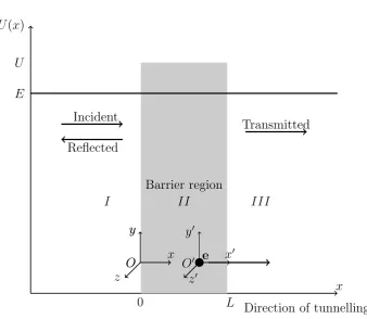
Figure 1: An electronewith kinetic energyEmoves along thex-axis and interacts with a rectangular barrier with heightU,U > E, and widthL
potential to the other side [14]. Some experimental investigations have supported a nonzero tunnelling time, while others supported a zero tunnelling time , [15, 16].
But for giving senses to the components of the time vector we have to opt to the nonzero tunnelling time and let us consider the case of one dimensional tunnelling of electron through a potential barrier.
U(x) =
0 when x <0
U when 0≤x≤L
0 when x > L
When both the widthLand the heightU are finite, a part of the quantum wave packet incident on one side of the barrier can penetrate the barrier boundary and continue its motion inside the barrier, where it is gradually attenuated on its way to the other side. A part of the incident quantum wave packet eventually emerges on the other side of the barrier in the form of the transmitted wave packet that tunneled through the barrier. How much of the incident waves can tunnel through a barrier depends on the barrier width L and its height U , and on the energy E of the quantum particle incident on the barrier. For such transmitted waves there are four widely used tunnelling times calculated by finding the transmission amplitude given by: T = |T|eiθ [18].The two of them are : Larmor time [19, 20], τ
LM and
Eisenbud-Wigner times [21],τEW. The first has been called resident or dwell
time:
τLM =−~∂θ
∂U (17)
The second has been called the passage time,
τEW =~
∂θ
∂E +
L
k (18)
An additional term,L/k is present inτEW, whereLand kare the barrier
width and electron velocity, respectively. This additional term corresponds to the propagation of the electron in the barrier region if that barrier were absent, and has to be added to get the total time [22], since the first term only gives a relative time shift [21].
However, the quantum tunnelling phenomena and the consideration of the time vector make to think that the Dirac equation inside the potential barrier (E < U) is not of the form (15) [24]. So, let us constructe the wave function of the electron inside the barrier in terms of the components of the time vector.
The energy vector E~ =
cp
0
mc2
before the barrier region will become
~
E =
cp
−U mc2
The timeT =pT02
3 +T102 andT20 can be qualified respectively as passage
time Tp = p
T02
3 +T102 and resident time Tr = T20. These three times, the
classical time T0 =p
T02 3 +T
02 1 +T
02
2 , the passage time Tp and the resident
time Tr evolve from the entrance to the outrance of the barrier region. But
according to the quantum tunnelling phenomena the classical time can not be observed, whereas at least one of the passage time and the resident time can be. Actually,
T0 >T
p T0 >Tr
All these times evolve from zero to positive values.
Let us search for θ in (17) and (18) in terms of τLM and τEW. From (17)
θ =−1
~
τLMU +K(E)
where K(E) is a function of E. Then,
∂θ
∂E =K
0
(E)
in substituting in (18)
K0(E) = 1
~
τEW −
1
~
L v
Using the relations p = qmv
1−v2
c2
and E = qmc2
1−v2
c2
(See for instance, [23]), we have
K0(E) = 1
~
τEW −
1
~
E
√
E2−m2c4L
and then
θ = 1
~(EτEW −U τLM −pL) +λ(L) (19)
with λ(L) independant of E and U, such thatU > E.
We will able to see the value of the constant λ(L) if a boundary conditions on the phase difference θ are determined. But, according to the couplings (9) and (11), for giving senses to the components of time vector, define the phase which evolves from the phase at x = 0 to x= L, inside the potential barrier, as
ϕII =−
1
~
E
q
T02 3 +T
02 1 −UT
0
2 −px
with at x=L, pT02
3 +T102 = τEW and T20 =τLM. Then, we have λ(L) = 0
ψI(x) =
1
−cp E+mc2
⊗ −1 1
e−~i
E√t02 3+t012−px
+A
1
cp E+mc2
⊗ −1 1 e−~i
E
√
t02 3+t
02 1+px
(x <0)
ψII(x) = B
1
−cp−iU
E+mc2
⊗ −1 1 e−~i
E√T02 3 +T
02 1 −UT
0 2−px
+C
1
cp−iU
E+mc2
⊗ −1 1 e−~i
E√T02 3 +T
02 1 −UT
0 2+px
(0< x < L) (20)
ψIII(x) =D
1
−cp E+mc2
⊗ −1 1 e− i ~
E√t02 3+t
02
1−px−EτEW+U τLM+pL
(L < x)
The form of each term of the wave function (20) inside the barrier is not like the one has been thought in [24]. It is a wave function solution, not of (1 + 1) spacetime Dirac equation particular case of (16), but a (1 + 2) spacetime Dirac equation.
In the case where the energy of the electron is higher than the value of the potential (E > U), the wave function inside the potential will be of the form
ψII(x) = A0
1
−cp−iU
E+mc2
⊗ −1 1 e− i ~
E√T02 3 +T
02 2 +T
02 1 −px
=A0
1
−cp−iU
E+mc2
⊗ −1 1 e− i ~
E√τ2
EW+τLM2 −px
because according to (8) the classical time t in the wave function (16) is
t =pT02 3 +T
02 2 +T
02 1 .
3.3
Discussion
If we choose +U as second component of the energy vector E~, the Larmor time τLM will be negative.
For both the two choices, according to the Feynman-St¨uckelberg interpreta-tion of the negative energy in the Dirac theory (See for instance [25]) it is not the electron which spends the resident time τLM but its antiparticle, a
positron.
Conclusion and Outlook
The energy vector in the Dirac theory has come when we would try to show the analogy between sign of helicity and the sign of energy, which we have then called sign of enginity. This energy vector need time vector whose components deserve physical senses.
The component of the time vector which occur when the electron takes an impulsion is not at all the responsible of the time dilation in special relativity. In the Dirac representation, for the tunnelling of the electron through a potential barrier the passage time can be defined as the magnitude of the projection of the time vector to the plan of first and third components of the time vector, whereas the dwell time can be defined as the second components of the time vector. They are respectively the Eisenbud-Wigner time and the Larmor time, τEW and τLM, at the potential barrier outrance. Then, for an
electron crossing a potential barrier the classical time
~
T0
=
p τ2
EW +τLM2
can not be observed, whereas the passage time τEW can be.
It has been shown from the coupling of the negative energy −U with the Larmor time τLM in the expression (19) of the phase difference that it is
not the electron which spends the resident time τLM but its antiparticle, a
positron.
References
[1] J.G. Muga, R. Sala Mayato and I.L. Egusquiza (Eds.), Time in Quan-tum Mechanics, Lect. Notes Phys. 734 (Springer, Berlin Heidelberg 2008), DOI 10.1007/978-3-540-73473-4.
[2] Bonacci E.,Hypothetical six-dimensional reference frames, International Journal of Mathematical Sciences & Applications, Vol. 5, No. 2, (July-December, 2015).
[3] C.A. Dartora, G.G. Cabrera,The Dirac Equation in Six-dimensional
SO(3,3) Symmetry Group and a Non-chiral Electroweak Theory,
Inter-national Journal of Theoretical Physics 49 (1) (2010) 51-61.
[4] E.A.B. Cole, Emission and absorption of tachyons in six-dimensional relativity, Physics Letters A75 (1-2)(1979) 29-30.
[5] D.R. Lunsford,Gravitation and Electrodynamics over SO(3,3), Interna-tional Journal of Theoretical Physics, 43 (1) (2004) 161-177.
[6] G. Ziino,On a straightforward experimental test for a three-dimensional time, Lettere Al Nuovo Cimento, 28 (16)(1980) 551-554.
[7] Raoelina Andriambololona, Rakotonirina C., A Study of the
Dirac-Sidharth Equation, EJTP 8, No.25, 177-182, 2011.
[8] P. A. M. Dirac, Proc. R. Soc. A117(778), (1928) 610; Proc. R. Soc. A126(801), (1930) 360.
[9] Schweber. S. S., Introduction to Relativistic Quantum Field Theory, (Harper and Row, New York), 1961, p 97.
[10] Rakotonirina C., Produit Tensoriel de Matrices en Th´eorie de Dirac, Th`ese de Doctorat de Troisi`eme Cycle (Supervised by Raoelina Andri-ambololona), Universit´e d’Antananarivo, Antananarivo, Madagascar, p 61, 2003, viXra : 1608.0232, https://vixra.org/abs/1608.0232.
[11] Xu, D., Wang, T. & Xue, X. Quantum tunnelling Time:
Relativistic Extensions. Found Phys 43, 12571274 (2013).
https://doi.org/10.1007/s10701-013-9744-2.
[13] Bjorken J.D. and Drell, S.D. (1964). Relativistic Quantum Mechanics, Mc-Graw Hill, New York, 1964, p.39.
[14] Razavy M., Quantum Theory of tunnelling, 2nd Edition, (World Scien-tific, Singapore, 2014), 2014.
[15] Shu Z., Hao X. L., Li W. D., Chen J., General way to define tunnelling time, Chin. Phys. B Vol. 28, No. 5 (2019) 050301, 2019.
[16] Hofmann C., Landsman A. S., Keller U., Attoclock revisited on electron
tunnelling time, (2019), Journal of Modern Optics, 66:10, 1052-1070,
DOI: 10.1080/09500340.2019.1596325, 2019.
[17] Hooge, Charles., BCIT Physics 8400 Textbook. (2018). https://opentextbc.ca/postsecondary/chapter/bcit/
[18] Landsman A. S., Keller U., Attosecond science and the tunnelling time problem, Physics Reports 547 (2015) 124.
[19] B¨uttiker M., Larmor precession and the traversal time for tunnelling, Phys. Rev. B, 1983. 27: p. 6178 - 6188
[20] Rybachenko V.F.,Time of Penetration of a Particle through a Potential Barrier, Sov. J. Nucl. Phys. 5 (1967) 635.
[21] Wigner, E.P., Lower Limit for the Energy Derivative of the Scattering Phase Shift, Physical Review, 1955. 98(1): p. 145-147.
[22] Hauge, E.H. and Støvneng J.A., Tunnelling times: a critical review, Rev. Mod. Phys., 1989. 61: p. 917 - 936.
[23] Baym G., Lectures on Quantum Mechanics, (W.A. Benjamin, Reading, 1976) Chapter 23.
[24] Rakotonirina C., Operator of sign of energy : Toward a consequence, Proceedings of the Eleventh International Conference in High-Energy Physics, HEPMAD 19, Antananarivo, Madagascar, October 14-20, 2019, edited by S. Narison, (2020).
[25] Thomson A., Modern Particle Physics, Cambridge University Press, 98, (2013).
[26] Bisht P. S., Jivan Singh and Negi O. P. S., Quaternionic Reformulation
of Generalized Superluminal Electromagnetic Fields of Dyons,