http://www.sciencepublishinggroup.com/j/ijbse doi: 10.11648/j.ijbse.20190702.13
ISSN: 2376-7227 (Print); ISSN: 2376-7235 (Online)
Analysis on Image Processing Technology-based Diabetic
Retinopathy
Hla Myo Tun
Department of Electronic Engineering, Yangon Technological University, Yangon, Myanmar
Email address:
To cite this article:
Hla Myo Tun. Analysis on Image Processing Technology-based Diabetic Retinopathy. International Journal of Biomedical Science and Engineering. Vol. 7, No. 2, 2019, pp. 45-60. doi: 10.11648/j.ijbse.20190702.13
Received: August 10, 2019; Accepted: August 29, 2019; Published: September 16, 2019
Abstract:
Diabetic retinopathy is a dangerous eye disease which causes the blindness widely in the human society. It arises due to high sugar level in the blood. The eye disease caused due to the diabetes is called diabetic retinopathy. The symptoms of diabetic retinopathy are red lesions such as microaneurysms (MA), intraretinal hemorrhages and bright lesions such as exudates, cotton wool spots and blood vessels. Microaneurysm (MA) is one of the features of the diabetic retinopathy. They are discrete, localized saccular distensions of the weakened capillary walls and appear as small round dark red dots on the retinal surface. According to the medical definition of MA, it is a reddish, circular pattern with a diameter λ is less than 125µm. Microaneurysms are mostly found near thin blood vessels, but cannot actually be located on the blood vessels. According to the number of microaneurysms, the diabetic retinopathy can be classified as mild stage, moderate stage and the severe stage. To detect the microaneurysms, the optic disc and the blood vessels are firstly detected because they are normal features of the image. And also, in the detection of microaneurysms the pre-processing stage is very important. In the pre-processing stage, the filtering techniques and the histogram equalization techniques are applied to reduce the effect of noise and uneven illumination cases. To detect the optic disc, blood vessels and the microaneurysms, the mathematical morphological method is applied. The result of this research can help in the screening of diabetic retinopathy.Keywords:
Image Processing Technology, Diabetic Retinopathy, Biomedical Engineering, Life Science, Medical Research1. Introduction
Nowadays the world's visions are threatened by the diabetic retinopathy. It is a dangerous eye disease that causes the blindness and blurs the vision of the human's eye. Diabetic retinopathy is the effect of diabetes on the eye. Diabetes arises due to the high sugar level in the blood. Basically, there are three types of diabetes: Type 1, Type 2 and Type 3 diabetes. Type 1 diabetes arises as a result of auto immune problem. The immune system of the body destroys the insulin producing beta cells in the pancreas leading to no or less production of the required insulin by the pancreas. Type 2 Diabetes includes non production of insulin or a situation known as insulin resistance. In this case, the muscles, fat and other cells do not respond to the insulin produced. Type 3 is also known as gestational diabetes and it only occurs during pregnancy. During this stage, the body resists the effect of insulin produced [1-2].
It can damage the small blood vessels of the eye and also
intraretinal hemorrhages and bright lesions such as exudates, cotton wool spots and blood vessels. Red lesions are the first clinically observable lesions indicating diabetic retinopathy. Therefore, their detection is indispensable for a prescreening system [3-5]. Microaneurysm (MA) is one of the features of the diabetic retinopathy. Retinal MAs are focal dilatations of retinal capillaries. This may also leads to big blood clots known as Hemorrhages [6]. They are discrete, localized saccular distensions of the weakened capillary walls and appear as small round dark red dots on the retinal surface. According to the medical definition of MA [5], it is a reddish, circular pattern with a diameter λ<125µm. Microaneurysms are mostly found near thin blood vessels, but they cannot actually locate on the blood vessels [5].
In this research, the image processing techniques are applied to identify the disease in order to reduce the blindness in the world. Early detection of the disease (Diabetic Retinopathy) can prevent the loss of vision. And also, it can help the ophthalmologist in the screening of diabetic retinopathy.
2. Colour Space Conversion
In digital image processing, images are either indexed images or RGB (Red, Green, and Blue) images. The input fundus image can be in RGBcolour space. An RGB image is an M x N x 3 array of colour pixels, where each colour pixel is a triplet corresponding to red, green and blue components of RGB image at specified special location. The range of value of an RGB is determined by its class. An RGB image of class double, has value in the range of (0 to 1), while class of uint8 is (0 to 255), similarly for the range (0 to 65535) is called class uint16. There are many other colour formats include: NTSC (luminance(Y), hue(I), saturation (Q) colour model), HIS (luminance(H), hue(I), saturation (S)) colour model), YCbCr (luminance(Y), hue(I), saturation (Q)) colour model), HSV (hue(H), saturation(S), Value(V)) colour model), CMY(cyan(C), Magenta(M), Yellow (Y) colour model) and CMYK(cyan(C), Magenta(M), Yellow (Y), black(K)) colour model [14].
2.1. NTSC Colour Spacing
In the NTSC color space, the luminance is the grayscale signal used to display pictures on monochrome (black and white) televisions. The other components carry the hue and saturation information. NTSC (luminance(Y), hue (I), saturation (Q)) colour system is used in television in United States. One of the advantages of this method is that the grayscale information is separate from colour data. The percentage of RGB components are given as red 29.9%, green 58.7% andblue 11.4%. The image data consists of three components luminance (Y), Hue (I) and Saturation (Q). The appropriate MATLAB function to use is: rgb2ntsc and the transformation matrix is given as below:
Y I Q
=
0.299 0.587 0.114 0.596 -0.274 -0.322 0.211 -0.523 0.312
R G B
(1)
2.2. The YCbCr Colour Spacing
In YCbCr (luminance(Y), hue (I), saturation (Q)) colour spacing, the luminance information is represented by a single component Y while the colour information is stored as two colour difference components Cb, Cr. If the input is uint8, YCBCR is uint8, where Y is in the range (16 to 235), and Cb and Cr are in the range (16 to 240). If the input is a double, Y is in the range (16/255 to 235/255) and Cb and Cr are in the range (16/255 to 240/255). If the input is uint16, Y is in the range (4112 to 60395) and Cb and Cr are in the range (4112 to 61680). The difference between the blue component and reference value component is called Cb while the difference between the red component and reference value is referred to as component Cr. This colour model is widely used in digital video. Appropriate MATLAB function for converting from RGB to YCbCr is: rgb2ycbcr. Convert from RGB to YCbCr uses the transformation matrix below:
Y I Q = 16 128 128 +
65.481 128.553 24.966 -37.797 -74.203 112.000
112.00 -93.786 -18.214 R G B
(2)
2.3. The HSV Colour Space
HSV (hue (H), saturation(S), Value (V)) colour space is generated by looking at the RGBcolour cube along the grey axis (the axis joining the black and white vertices) resulting in a hexagonally shaped colour palette. RGB is an m-by-n-by-3 image array whose three planes contain the red, green, and blue components for the image. HSV is returned as an m-by-n-by-3 image array whose three planes contain the hue, saturation, and value components for the image. This colour system is based on the cylindrical coordinates, thereby making conversion from RGB to HSV similar to a mapping RGB coordinate values to cylindrical coordinates function. Appropriate MATLAB function for converting RGB to HSV is: rgb2hsv.
2.4. The CMY and CMYK Colour Spaces
C M Y = 1 1 1 -R G B (3)
2.5. HIS Colour Space
HSI means hue saturation and intensity. In this colour model space, the intensity component is decoupled from colour carrying information (hue and saturation) in colour image, hence an ideal tool for the development of image processing algorithms. The HSI space consists of a vertical intensity axis and the locus of colour points that lie on a plane perpendicular to this axis, as the plan move up and down the intensity axis. The important components of HSIcolour space are the vertical intensity axis and the length of the vector to the colour point and the angle this vector makes to the red axis. The transformation equations used in the conversion of RGB to HSI are as follow:
H component of each RGB pixel is obtained using the following equation
θ If B G H
360 θ If B G
≤
=
− >
(4)
[
]
1 2 1 ( ) ( ) 2 cos 1 2 ( ) ( )( )R G R B
R G R B G B
θ − − + − = − + − − (5)
Saturation component is
S=1- 3
(r+g+b) min(R,G,B) (6)
Finally, the intensity component is I=1
3 R+G+B (7)
3. Histogram Equalisation
Histogram equalization technique is used to overcome the effects of uneven illumination case. It enhances the contrast of images by transforming the values in an intensity image so that the histogram of the output image approximately matches a specified histogram. The purpose of standard histogram equalisation scheme is to optimize the overall contrast of the image by obtaining a uniform histogrammed version of the gray image. It attempts to equalize the probability of occurrence of all the gray values of the image. SHE employs a monotonic, non-linear mapping that assigns a new intensity value to each of the pixels based on following computation: The probability density function of a digital image of “n” pixels with gray level range [0, L-1] is given by equation (1)
nk
P(r )
k
=
n
(8)Where 0≤rk≤1 and k = 0, 1, …, L – 1, and rk stands for the
kth gray level, nk represents the number of pixels in the kth level and n is the total pixel count. The transformation mapping of the gray level rk to a new level sk based on a cumulative distribution function is obtained using equation (2), which may be expressed as:
k
nj
k
S
T(r )
P(rj)K 0,1,...,L 1
k
k
n
j 0
j 0
=
=
∑
=
∑
=
−
=
=
(9)
Where 'T' stands for the transformation function. This method is particularly useful, where, both background and foreground are dark and represented by a set of narrow gray values. Images acquired from fluorescence oscilloscope are often very low in contrast, which is evident from their histograms that are narrow and concentrated only to certain gray level values. Retinopathy images contain minute details of the lesions and intra-retinal occlusions that get obscured due to limited contrast, and hence, are not easily presented before doctors. This may lead to delayed diagnosis and even wrong treatment. Histogram equalization plays an important role in several such cases, but leaves local changes in contrast unconsidered [8].
3.1. Contrast Limited Adaptive Histogram Equalisation (CLAHE)
The CLAHE algorithm is defined to function adaptively on the image to be enhanced, unlike standard histogram equalization. It optimizes the contrast enhancement on local image data in a divide and conquer manner and hence efficiently tackles the global noise. In other words, the basic idea of the algorithm is to divide the image into a number of small, non-overlapping contextual regions, called “Tiles”. The neighboring tiles are then combined using bilinear interpolation to eliminate artificially induced boundaries. The contrast, especially in homogeneous areas, can be limited to avoid amplifying any noise that might be present in the image [8]. The main objective of this method is to define a point transformation within a local fairly large window with the assumption that the intensity value within it is a stoical representation of local distribution of intensity value of the whole image. The local window is assumed to be unaffected by the gradual variation of intensity between the image centres and edges. The point transformation distribution is localised around the mean intensity of the window and it covers the entire intensity range of the image. Consider a running sub image W of N X N pixels centred on a pixel P (i, j), the image is filtered to produced another sub image P of (N X N) pixels according to the equation below
w w n w w P
(P)-
(Min)
255
(Max)-
(Min)
ϕ
ϕ
ϕ
ϕ
=
×
(10)w 1 w w (P)
µ
P
1 exp
ϕσ
− −
= +
(11)and Maxand Min are the maximum and minimum intensity values in the whole image, while µw andσw indicate the
local window mean and standard deviation which are defined as: w 2 (i,j) (k,i) 1 µ P(i,j) N ∈
=
∑
(12)(
)
2w 2 w
(i,j) (k,i) 1 P(i,j)-µ N
σ
∈=
∑
(13)3.1.1. Thresholding
The thresholding method is a simple shape extraction technique and applied to detect the desire area. Therefore, the resulting image was binarized by thresholding.
1,f(x,y) T
g(x,y)
0,f(x,y) T
≥
=
<
(14)Where, g (x, y) is the binary value of the pixel and f (x, y) is gray value of a pixel in the result image of image enhancement.
The threshold value is depended on automated selection by using the Otsu algorithm. Otsu’s method [9] is one of the most popular techniques of optimal thresholding; there have been surveys [10-13] which compare the performance different methods can achieve. Essentially, Otsu’s technique maximizes the likelihood that the threshold is chosen so as to split the image between an object and its background. This is achieved by selecting a threshold that gives the best separation of classes, for all pixels in an image. The graythresh function uses Otsu's method, which chooses the threshold to minimize the intraclass variance of the black and white pixels.
The equations of the Otsu's Algorithm are as follow: σ2 Between(T)=wB(T)wo(T)[µB(T)-µo(T)]
2
(15)
wB T =∑ p i T-1
i=0 (16)
µB T =∑T-1i=0 ip ip(i) (17)
w0 T =∑ p i L-1
i=T (18)
µ0 T =∑L-1i=T ip ip(i) (19)
where, σ2Between(T)=Between-class variance
w=weight, B=background of the image, o=object of image µ=combined mean,
T=threshold value
3.1.2. Filtering Techniques
An image is often corrupted by noise in its acquisition and transmission. Noise is any unwanted information that contaminates an image. Noise appears in images from a variety of sources. The goal of denoising is to remove the noise while retaining as much as possible the important signal features. Denoising can be done through filtering, which can be either linear filtering or non-linear filtering.
3.1.3. Median Filter
The median filter is a nonlinear filter, which can reduce impulsive distortions in an image and without too much distortion to the edges of such an image. It is an effective method that of suppressing isolated noise without blurring sharp edges. Median filtering operation replaces a pixel by the median of all pixels in the neighbourhood of small sliding window. The operation of the median filter is – first arrange the pixel value in either ascending or descending order and then compute the median value of the neighborhood pixels. It gives better results than the neighbourhood averaging in the case where noise is of impulsive nature. The advantage of a median filter is that it is very robust and has the capability to filter only outliers and is thus an excellent choice for the removal of especially salt and pepper noise and horizontal scanning artifacts. The median filter is realized in MATLAB by the function medfilt 2.
3.1.4. Averaging Filter
The averaging filter is also used to reduce the effect of noise in image. The operation of the averaging filter is each pixel gets set to the average of the pixels in its neighborhood. The effect of averaging is to reduce noise; this is its advantage. An associated disadvantage is that averaging causes blurring which reduces detail in an image. It is also a low-pass filter since its effect is to allow low spatial frequencies to be retained, and to suppress high-frequency components. A larger template, say 3 × 3 or 5 × 5, will remove more noise (high frequencies) but reduce the level of detail. The size of an averaging operator is then equivalent to the reciprocal of the bandwidth of a low-pass filter that it implements.
3.1.5. Wiener Filter
The wiener filter tries to calculate the optimal estimate of the original image by enforcing a minimum mean-square error constraint between estimate and original image. The wiener filter is an optimum filter. The objective of the wiener filter is to minimize the mean square error. A wiener filter has the capability of handling both the degradation function as well as noise. The wiener filter requires to know the power spectral density of the original image which is unavailable in practice. Wiener filter can be done by using wiener2 function.
3.2. Mathematical Morphological Method
operations include dilation, erosion, opening, closing and skeletonization etc. Mathematical morphology analyses images by using operators developed using set theory [14-16]. It was originally developed for binary images and was extended to include grey-level data. The word morphology concerns shapes: in mathematical morphology the image can be processed images according to shape, by treating both as sets of points. In this way, morphological operators define local transformations that change pixel values that are represented as sets.
3.2.1. Dilation
Dilation is a process that thickens objects in a binary image. The extent of this thickening is controlled by the Structuring Element (SE) which is represented by a matrix of 0s and 1s.
Mathematically, dilation operation can be written in terms of set notation as below
A ⊕ As z| A’s z ∩ A Φ (20) Where Φ is an empty element and As is the structuring element. The dilation of A by As is the set consisting of all structuring element origin locations where the reflected and transmitted As overlaps at least some portions of A. Dilation operation is commutative and associative.
3.2.2. Erosion
Erosion shrinks or thins the objects in a binary image by the use of structuring element. The mathematical representation of erosion is as shown below.
A Θ As z| As z ∩ Ac Φ (21) Erosion is performed in MATLAB using the command imerode (Image Name, SE). One of the most common applications of this is to remove noise in thresholded images.
3.2.3. Opening and Closing
In image processing, dilation and erosion are used most often and in various combinations. An image may be subjected to series of dilations and or erosions using the same or different SE. Closing and opening operators are generally used as filters that remove dots characteristic of pepper noise and to smooth the surface of shapes in images. These operators are generally applied in succession and the number of times they are applied depends on the structural element size and image structure. The combination of this two principles leads to morphological image opening and morphological image closing.
Morphological opening can be described as an erosion operation followed by a dilation operation. Morphological opening of image X by Y is denoted by X οY, which is erosion of X by Y followed by dilation of the result obtain by Y closing and opening
X οY X ⊕ Y ΘY (22)
X • Y XΘY ⊕ Y (23)
Morphological closing can also be described as dilation operation followed by erosion operation. Morphological Closing of Image X by Y is denoted by X •Y, which is dilation of X by Y followed by erosion of the result obtained by Y. Image opening and image closing and are implemented in MATLAB by the use of imopen(image name) and imclose(image name) respectively.
3.2.4. Skeletonization
Skeletonization is another way to reduce binary image objects to a set of thin strokes that can display important information about the shape of the original objects. Skeletonization is similar to thinning, except that it maintains more information about the internal structure of objects with it being 1 pixel thick. To reduce all objects in an image to lines, without changing the essential structure of the image, use the bwmorph function. This process is known as skeletonization.
4. Implementation of the Proposed
System
In this setion, the stages about the optic disc detection, the blood vessels detection and the microaneurysms detection are discussed. These stages are very important because the ophthalmologist can use the results in the detection of diabetic retinopathy. The general flow chart of the detection of diabetic retinopathy is shown in Figure 1.
4.1. Pre-Processing Stage
The pre-processing stage is the necessary step for the next stages. In this stage, the noise contained in the image is removed and reduced the uneven illumination case. The pre-processing stage includes the following steps:
a)Colour Space Conversion b)Filtering Techniques
c)Contrast Limited Adaptive Histogram Equalisation
4.2. Colour Space Conversion
The colour space conversion is an essential step for the next processes. For example, RGBcoulour space is converted into HSIcolour space for optic disc detection and RGBcolour space is converted into gray scale image for blood vessels detection.
4.3. RGB to HSI Conversion
The first stage of the pre-processing stage is the colour space conversion. The input image can be either RGB or other colour formats. So, the input image is converted into Hue, Saturation and Intensity (HSI) color space for the optic disc detection because HSIcolour space is more appropriate to separate the intensity component from the other two components. And also, the information needed for the further process is contained in the intensity component. Therefore, the colour space conversion RGB to HSI is the necessary step for the detection of the diabetic retinopathy. After that the filtering technique and the histogram equalization technique are applied for the image enhancement purpose. The conversion of RGB to HSI has been discussed fully in the previous setion. The input RGB image and the outputHSI image are shown in Figure 2 and Figure 3.
Figure 2. Original RGB Image.
Figure 3. HSI Image (RGB to Gray Scale Conversion).
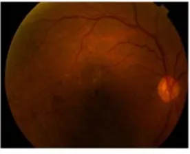
Figure 4. Original RGB Image.
For the blood vessels detection, the original RGB image is converted into gray scale image because that colour space is more suitable to detect the blood vessels than the other colour space. The conversion of RGB images to grayscale is by eliminating the hue and saturation information while retaining the luminance. The input image and the result of RGB to Gray scale image are shown in Figure 4 and Figure 5.
Figure 5. Gray Scale Image.
4.4. Filtering Techniques
The noise contained in the image is reduced by using filtering techniques such as median filter, wiener filter and averaging filter.
4.5. Median Filter
Median filter is used in the pre-processing stage in order to remove the noise which contains in the image. The median filter is a non-linear filter type and which is used to reduce the effect of noise without blurring the sharp edge. The operation of the median filter is – first arrange the pixel values in ascending order and then compute the median value of the neighborhood pixels. The result of the median filter is used in the further processes and using the default 3-by-3 neighborhood.
Figure 7. Result of Median Filter.
4.6. Wiener Filter
The wiener filter is used to minimize the mean square error between input and output image. The objective of the wiener filter is to minimize the mean square error. A wiener filter has the capability of handling both the degradation function as well as noise. The wiener filter requires to know the power spectral density of the original image which is unavailable in practice. Wiener filter can be done by using wiener2 function using neighborhoods of size m-by-n to estimate the local image mean and standard deviation and m and n default to 3. The result of the wiener filter is shown in Figure 9. The equation of the wiener filter is
1 2 ff 1 2
1 2
2
1 2 ff 1 2 ηη 1 2
(ω ω
H*(ω ,ω ) S (ω ,ω )
,
)
H(ω ,ω )
S (ω ,ω ) S (ω ,ω )
×
=
×
+
G (24)
where, Sff ω1, ω2 and SȠȠ ω1, ω2 are Fourier transform of the image covariance and noise covariance.
Figure 8. Image with Noise.
Figure 9. Result of Wiener Filter.
4.7. Averaging Filters
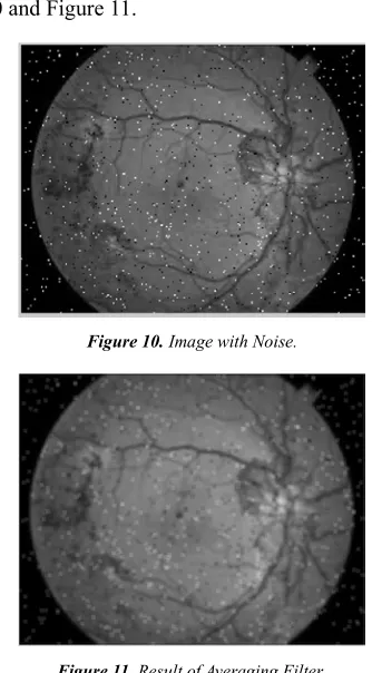
Averaging filter is useful for removing grain noise from a photograph. Each pixel gets set to the average of the pixels in its neighborhood. The averaging filter is also known as the mean filter. The median filter is a non-linear while the averaging filter is a linear one. The effect of averaging is to reduce noise; this is its advantage. An associated disadvantage is that averaging causes blurring which reduces detail in an image. It is also a low-pass filter since its effect is to allow low spatial frequencies to be retained, and to suppress high-frequency components. A larger template, say 3 × 3 or 5 × 5, will remove more noise (high frequencies) but reduce the level of detail. The size of an averaging operator is then equivalent to the reciprocal of the bandwidth of a low-pass filter that it implements. The operation of the averaging filter is- find the average of the neighborhood pixels and replace the value and using the default 3-by-3 neighborhood. The image with noise and the result image are shown in Figure 10 and Figure 11.
Figure 10. Image with Noise.
Figure 11. Result of Averaging Filter.
According to the Table 1, the median filter is used to reduce the effect of noise and filtering purpose.
Table 1. Performance Comparison of Filtering Techniques.
Types of Filter MSE PSNR
Median Filter 2.6338 43.9249
Averaging Filter 18.1549 24.7432
Wiener Filter 4.5840 41.5183
2
1 1 1
( ( , ) ( , )) M N
i j
MSE x i j y i j
MN = =
=
∑∑
− (25)2
10
(2 1) 10 log
n
PSNR
MSE
−
=
(26)
Where, x(i, j)=the original image Y(i, j)=the output filtered image
M × N=the number of rows and columns in the input images
n=number of bits
The lower the value of MSE, the lower the error. The higher the PSNR, the better the quality of the compressed or reconstructed image.
4.8. Histogram Equalisation
One of the problems associated with fundus images is uneven Illumination. Some areas of the fundus images appear to be brighter than the other. Areas at the centre of the image are always well illuminated, hence appears very bright while the sides at the edges or far away are poorly illuminated and appears to be very dark. In fact the illumination decreases as distance form the centre of the image increase. The purpose of standard histogram equalisation scheme is to optimize the overall contrast of the image by obtaining a uniform histogrammed version of the gray image. It attempts to equalize the probability of occurrence of all the gray values of the image. The original images and the results of standard histogram equalization are shown in Figure 12 to Figure 15.
Figure 12. Original Image.
Figure 13. Histogram of Original Image.
Figure 14. Standard Histogram Equalisation Image.
Figure 15. Histogram of Image after Standard Histogram Equalisation.
4.9. Contrast Limited Adaptive Histogram Equalisation
Most of the input fundus images can face with the problem of uneven illumination. Due to the uneven illumination case, some area of the fundus images appear brighter than the other area for example, at the center of the image is always bright and sharp but the sides at the edges are dark and poorly illuminated. To reduce the uneven illumination case, the contrast limited adaptive histogram equalization (CLAHE) is applied. The main objective of this method is to define a point transformation within a local fairly large window with the assumption that the intensity value within it is a stoical representation of local distribution of intensity value of the whole image.
As a result of this adaptive histogram equalization, the dark area in the input image that was badly illuminated has become brighter in the output image while the side that was highly illuminated remains or reduces so that the whole illumination of the image is same. The original images and the results of the adaptive histogram equalization are shown in Figure 16 to Figure 19.
Figure 17. Histogram of Original Image.
Figure 18. Adaptive Histogram Equalization Image.
Figure 19. Histogram of Image after Adaptive Histogram Equalisation.
4.10. Segmentation Stage
The segmentation stage is the important step in the detection of diabetic retinopathy because the ophthalmologist can detect the disease easily by using the results of the segmentation stage.
4.10.1. Optic Disc Detection
The optic disc detection is the important step for the further processes. The optic detection is useful because it can reduce the false positive detection of the exudates because the optic disc and the exudates are the brightest portion of the image. The optic disc can be seen as the elliptical shape in the eye fundus image. Its size varies from one person to another, between one-tenth and one-fifth of the image. The maximum diameter of optic disc can be of 2mm. The
mathematical morphology methods are applied to detect and eliminate the optic disc. The morphological operations include dilation, erosion, opening, closing and so on. The general procedure of the optic disc detection is shown in Figure 20. To detect the optic disc, first the input RGB image is converted into HSIcolour space, the median filter and the histogram equalization techniques are used to reduce the noise and uneven illumination cases. These results have been discussed and also these results are used in the detection of the optic disc. The closing operator is applied to the preprocessed image, when the closing operator is used the choice of structuring element is important. The closing is a dilation followed by erosion that joins very close objects together. And then, morphological reconstruction is applied to the image. Morphological reconstruction can be thought of conceptually as repeated dilations of an image, called the marker image, until the contour of the marker image fits under a second image, called the mask image. In morphological reconstruction, the peaks in the marker image "spread out," or dilate. To detect the optic disc, the Otsu’s algorithm is applied to the difference between the original image and the reconstructed image. The original image and the optic disc detected image are shown in Figure 21 and Figure 22.
Figure 21. HSI Image.
Figure 22. Optic Disc Detected Image.
4.10.2. Blood Vessels Detection
Figure 23. General Procedure for the Blood Vessels Detection.
The blood vessels detection is also important as the optic disc detection because the optic disc and the blood vessels are the normal features of the image. The appearance of blood vessel in a retinal image is complex and having low contrast. In fundus retinal image, the blood vessels appeared as a network like structure. The main blood vessels originate from the center of the OD and grow to different branches. The general procedure for the blood vessels detection is shown in Figure 23. To detect the blood vessels, first the
input image is converted into grayscale image due to strengthen the appearance of the blood vessels. Same as the optic disc detection, the median filter and the histogram equalization techniques are used for the same purposes in the pre-processing stage. Then, the closing operator is applied and then the filling operator is used to fill holes in the blood vessels. Therefore, the blood vessels appear strongly in the image and then the Otsu algorithm is applied to detect the blood vessels. The optic disc detection and the blood vessels detection are necessary steps for the detection of diabetic retinopathy. The general flow chart for the blood vessel detection is shown in Figure 23.
The original image and the result image are shown in Figure 24 and Figure 25. By using the results of the optic disc detection and the blood vessels detection, the ophthalmologist can detect the disease easily.
Figure 24. Original image.
Figure 25. Blood Vessels Detected Image.
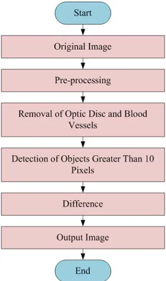
4.10.3. Microaneurysm Detection
Microaneurysm (MA) is one of the features of the diabetic retinopathy. Retinal MAs are focal dilatations of retinal capillaries. This may also leads to big blood clots known as Hemorrhages. The general flow chart for the microaneurysms detection is shown in Figure 26.
the image set of size 752 × 500 pixels, the size of a MA is about 10 pixels. Microaneurysms are mostly found near thin blood vessels, but they cannot actually locate on the blood vessels. Image processing of color fundus images is more challenging and hard to distinguish due to the different ‘distractors’ within the image that may be confused with diabetic lesions eg., small vessels, intersection of two thick vessels or a few very thin vessels, choroidal vessels, reflection artefacts and leads to misinterpretation to the detectors.
Figure 26. General Procedure for the Microaneurysms Detection.
To detect the microaneurysms, the optic disc and the blood vessels are eliminated from the image firstly because they are the normal feature of the image. According to the number of microaneurysms the disease can be classified as mild, moderate and severe cases. To find an MA by its diameter and isolated connected red pixels with a constant intensity value, and whose external border pixels all have a higher value in the green plane of a RGBimage. A preprocessed retinal image was used as the primary image for MA detection. The extended-minima transform is applied to the fE
image. This transformation is a thresholding technique that brings most of the valleys to zero. The extended minima transform is applied on the fE image with threshold value α2.
fE=Extended minima transform(fp, α2) (27)
Where fE is the transformed image and fp is preprocessed
imageThe selection of threshold is most important. Where the higher value of α2 will decrease the number of regions and a lower value of α2 will increase the number of regions.
Figure 27. The Input Retinal Image.
Figure 28. The Output Retinal Image (No DR).
Figure 29. The Input Retinal Image.
Figure 31. The Input Retinal Image.
Figure 32. The Output Retinal Image (Moderate Stage of DR).
Figure 33. The Input Retinal Image.
Figure 34. The Output Retinal Image (Severe stage of DR).
5. Experimental Results
In this setion, the results of this research will be presented and discussed. According to the results of the microaneurysms detection, the fundus image can be classified as normal and abnormal. And also, the disease can be classified as mild stage, moderate stage and serve stage depending on the numbers of microaneurysms.
The criteria used for grading the diabetic retinopathy are described in Table 2.
Table 2. Criteria used for grading the diabetic retinopathy.
Numbers of microaneurysms (MA) Stage of Disease (DR)
MA=0 no DR (Grade 0)
1≤MA≤5 Mild(Grade 1)
5<MA<15 Moderate(Grade 2)
MA≥15 Severe(Grade 3)
Performance metrics was done by comparing the segmentation results to the reference image. There are four values resulted from the validation procedure, true positive (TP), false positive (FP), true negative (TN) and false negative (FN). TP is a number of pixels correctly detected as microaneurysms (MA), FP is a number of pixels incorrectly flagged, TN is a number of pixels correctly detected as non MA and FN is a number of pixels incorrectly flagged as non MA.
The correct and incorrect percentages of this research can be calculated by using following equations:
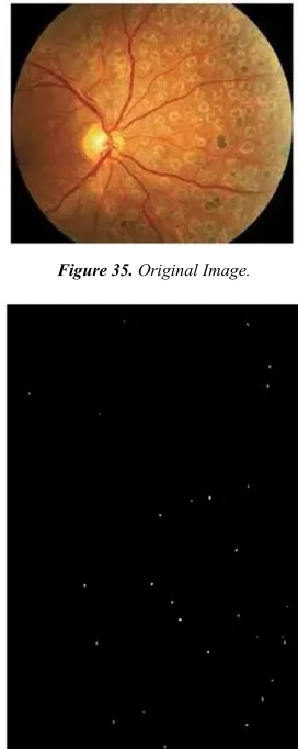
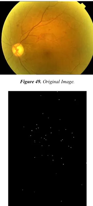
Correct=[TP+TN]/[TP+TN+FN+FP] (28) Incorrect=[FP+FN]/[TP+TN+FN+FP] (29) Figures 35 and 36 show the original image and the microaneurysms (MA) detected image. According to the medical definition, if the number of MA is greater than 15 the disease is assigned as severe stage. And also, the ophthalmologist identified the disease as the severe case.
Figure 35. Original Image.
Figures 37 and 38 show the original image and the result image of the research. The algorithm identified the disease as the severe case and also the ophthalmologist determined the disease as the severe case.
Figure 37. Original Image.
Figure 38. Image of Detected Microaneurysms.
Figure 39 is the healthy retinal image and the algorithm identified as no disease too. The result image is shown in Figure 40. The ophthalmologist identified the Figures 41 and 42. as mild stage of the diabetic retinopathy (DR) and the algorithm identified as the mild stage too.
Figure 39. Original Image.
Figure 40. Image of Detected Microaneurysms.
Figure 41. Original Image.
Figure 42. Image of Detected Microaneurysms.
than 15 and identified as severe stage of DR and the ophthalmologist identified the same. For Figures 45 and 46, the ophthalmologist identified the disease as the severe stage and the algorithm identified as moderate stage. For Figures 47 and 48, ophthalmologist identified the disease as severe case and the algorithm also identified as moderate stage of DR. For Figures 49 and 50, the ophthalmologist and the algorithm identified the disease as the severe stage.
Figure 43. Original Image.
Figure 44. Image of Detected Microaneurysms.
Figure 45. Original Image.
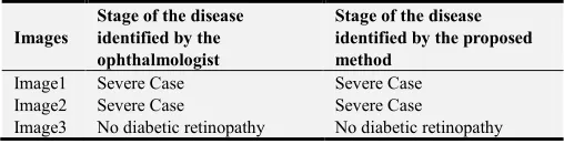
Table 3. Performance of the Proposed Method to Identify the Severity of the Diseasefor Corresponding Input Images.
Images
Stage of the disease identified by the ophthalmologist
Stage of the disease identified by the proposed method
Image1 Severe Case Severe Case Image2 Severe Case Severe Case
Image3 No diabetic retinopathy No diabetic retinopathy
Images
Stage of the disease identified by the ophthalmologist
Stage of the disease identified by the proposed method
Image4 Mild Case Mild Case
Image5 Severe Case Severe Case Image6 Severe Case Moderate Case Image7 Severe Case Moderate Case Image8 Severe Case Severe Case
Figure 46. Image of Detected Microaneurysms.
Figure 47. Original Image.
Figure 49. Original Image.
Figure 50. Image of Detected Microaneurysms.
Table 3 shows the results of the detection of microaneurysms and the stages of the diabetic retinopathy. The research for the microaneurysms detection was applied to 21 retinal images of which 18 images with severe case and 3 images with other cases. The correct and incorrect percentages of this research can be calculated by using following equations:
Correct= [TP+TN]/[TP+TN+FN+FP] (30) Incorrect= [FP+FN]/[TP+TN+FN+FP] (31) The percentages for the correct and incorrect detection are 77% and 23%.
6. Discussions
The preprocessing stage is the important step for the further process. The noise contained in the image was removed by using the filtering techniques. The median filter is a non-linear filter type and which is used to reduce the effect of noise without blurring the sharp edge. The wiener filter is used to minimize the mean square error between input and output images. The wiener filter requires to know the power spectral density of the original image which is unavailable in practice. This is a major drawback of the wiener filter. The averaging filter is useful for removing grain noise from a photograph. The averaging causes blurring
which reduces details in an image. According to the values of MSE and PSNR, the median filter is the most suitable for the noise removal purpose. The lower the value of MSE, the lower the error. The higher the PSNR, the better the quality of the compressed or reconstructed image. The microaneurysms are one of the features of the diabetic retinopathy. According to the number of microaneurysms, the stages of the disease can be classified. The correct and incorrect percentages of the detection of diabetic retinopathy are 77% and 23%. This research only focuses on the microaneurysms and there still need to detect the exudates to get the exact results. The exudates are also the symptom of the diabetic retinopathy. This method doesn't need the highly efficient computer so it is suitable for rural area in developing countries. But, for the poor quality images this method cannot be detected and the number of microaneurysms cannot be counted automatically. The outcomes of this research work are high level results by comparing with the results of the study [2]. The accuracy of this research work is also high and the performance of the proposed system is also elevatedfor real applications.
7. Conclusion
The diabetic retinopathy is a dangerous eye disease and early detection of it can prevent the loss of vision. This research can help the ophthalmologist in the screening of diabetic retinopathy. First, the noise contained in the image and the uneven illumination case was reduced in the pre-processing stage. Then, the mathematical morphology method was used to detect the optic disc and the blood vessels. Detection of the optic disc and the blood vessels are the essential steps because the optic disc and the blood vessels are the normal feature of the image. And then, the microaneurysms can be detected and the results can help the ophthalmologist in the screening of diabetic retinopathy. According to the number of microaneurysms, the diseases can be classified as mild case, moderate case and severe case.
References
[1] Anonymous, “The Berries: Diabetic Retinopathy”, Accessed
August 4, 2013,
http://www.theberries.ns.ca/ARchives/2006Winter/diabetic_re tinopathy.html.
[2] Anonymous, “My Eye World: Eye Structure and function.”
Referenced, August 2nd 2013,
http://www.myeyeworld.com/files/eye_structure.htm. [3] SujithKumar S B, and Vipula Singh “Automatic Detection of
Diabetic Retinopathy in Non-dilated RGB Retinal Fundus Images” International Journal of Computer Applications (0975-888) Vol 47–19, June 2012.
[5] BálintAntal, IstvánLázár, AndrásHajdu “Novel Approaches to Improve Microaneurysm Detection in Retinal Images” Proceedings of the 8th International Conference on Applied Informatics Eger, Hungary, January 27–30, 2010. Vol. 1. pp. 149–156.
[6] B. Dupas, T. Walter, A. Erginay et al., “Evaluation of automated fundus photograph analysis algorithms for detecting microaneurysms, haemorrhages and exudates, and of a computer-assisted diagnostic system for grading diabetic retinopathy,” Diabetes & Metabolism 36 (3), 2010, pp. 213-220.
[7] B´alintAntal, and Andr´asHajdu “Improving microaneurysms detection in color fundus images by using an optimal combination of preprocessingmethods and candidate extractors” 18th European Signal Processing Conference (EUSIPCO-2010) Aalborg, Denmark, August 23-27, 2010. [8] S. Jayaraman: Digital Image Processing; 3 edition ISBN(10):
0-07014479-6: 2010.
[9] Lei Zhang, Qin Li, Jane You, and David Zhang, “A Modified Matched Filter With Double-Sided Thresholding for Screening Proliferative Diabetic Retinopathy”, IEEE Transactions On Information Technology In Biomedicine, Vol. 13, No. 4, pp. 528-534, July 2009.
[10] Sight Savers: The structure of the human eye. Accessed,
August 2, 2006, from website:
http://www.sightwavers.or.uk/html/eyeconditions/huma_eye_d etailed.htm.
[11] Xiaohui, Z., and Chutatape, O., “Detection and classification of bright lexions in colour fundus images”, Int. Conference on Image Processing, Vol 1, pp 139-142, Oct 2004.
[12] Vallabha, D., Dorairaj, R., Namuduri K. R., and Thompson, H., "Automated Detection and Classification of Vascular Abnormalities in Diabetic Retinopathy", 38th Asilomar Conference on Signals, Systems and Computers, November 2004.
[13] Joes Staal, Michael D. Abràmoff, MeindertNiemeijer, Max A. Viergever, and Bram van Ginneken, “Ridge-Based Vessel Segmentation in Color Images of the Retina”, IEEE Transactions On Medical Imaging, Vol. 23, No. 4, pp. 501-509, April 2004.
[14] Rafael C. Gonzalez and Richard E. Woods.“Digital Image Processing using MATLAB”, 2nd edition. Prentice Hall, 2002. ISBN 0-201-18075-8.
[15] Junichiro Hayashi, TakamitsuKunieda, Joshua Cole, Ryusuke Soga, Yuji Hatanaka, Miao Lu, Takeshi Hara and Hiroshi Fujita: A development of computer-aided diagnosis system using fundus images. Proceeding of the 7th International Conference on Virtual Systems and MultiMedia (VSMM 2001), pp. 429-438 (2001).