Automated Parasite’s Detection in Microscopic Images of Stools Using Distance Regularized Level Set Evolution Initialized with Hough Transform

http://www.sciencepublishinggroup.com/j/ijbecs doi: 10.11648/j.ijbecs.20190503.13

ISSN: 2472-1298 (Print); ISSN: 2472-1301 (Online)

Automated Parasite’s Detection in Microscopic Images of

Stools Using Distance Regularized Level Set Evolution

Initialized with Hough Transform

Oscar Takam Nkamgang

1, 2, *

, Daniel Tchiotsop

2

, Beaudelaire Saha Tchinda

2

,

Hilaire Bertand Fotsin

1

1

Research Unity of Condensed Matter Electronics and Signal Processing (URMACETS), Department of Physics, Faculty of Science, University of Dschang, Bandjoun, Cameroon

2

Research Unity of Automatic and Applied Informatics (URAIA), University Institute of Technology Fotso-Victor, University of Dschang, Bandjoun, Cameroon

Email address:

*

Corresponding author

To cite this article:

Oscar Takam Nkamgang, Daniel Tchiotsop, Beaudelaire Saha Tchinda, Hilaire Bertand Fotsin. Automated Parasite’s Detection in

Microscopic Images of Stools Using Distance Regularized Level Set Evolution Initialized with Hough Transform. International Journal of Biomedical Engineering and Clinical Science. Vol. 5, No. 3, 2019, pp. 45-58. doi: 10.11648/j.ijbecs.20190503.13

Received: August 20, 2019; Accepted: September 16, 2019; Published: October 23, 2019

Abstrat:

Background and purpose: The analysis of biomedical microscopic images is carried out manually in medical laboratories. The manual analysis of clinical images lets to both repetitive tasks and management of huge amounts of data. This is tedious and times consuming for laboratory technicians. Inevitably, it is also prone to human errors. Our objective in this work is to contribute to the automation of the analysis of microscopic images of stools using Distance Regularized Level Set Evolution automatically initialized by Hough transform. Method: We firstly converted the microscopic images to edge maps using canny algorithm. Next, we located the parasite through circular Hough transform and draw circles around them. Those circles stand as initial contours of DRLSE. The contours evolve until they fit the boundaries of the parasites. The final extraction is performed using a complementary method based on the signed distance character of the level set function. Results: The Distance Regularized Level Set Evolution has been automatically initialized. We applied our method to the detection of intestinal parasites in microscopic images. Experimental results show accurate, efficient and less time consuming of our scheme compared to others recently proposed in the literature. Conclusion: This is a notable contribution to the automation of stools examination in the medical laboratories. In forthcoming works, we plan to include this segmentation process in an expert system of parasitic diseases diagnosis.

Keywords:

Parasitosis Diagnosis Automation, Microscopic Image, Automated Segmentation, Distance Regularized Level Set (DRLSE), Hough Transform

1. Introduction

The parasitic diseases are responsible of considerable morbidity and mortality worldwide. The laboratory test plays a very significant role in the diagnosis process and constitutes the key step in the therapeutic decision. Such laboratories tests are brought out by comparing items shapes with well known parasites itemized by World Health Organization (WHO) [1]. The identification is done by

extraction. Two principal approaches are generally employed. Some approaches take into account color and texture information and combine with learning techniques [5]. The second group of methods quantify the presence of a boundary at a given image location through local measurements and model edges as sharp discontinuities in the brightness channel. Such family that uses a ‘’gradient filter’’ for edge detection includes: the Robert’s Cross operator [6], the Laplacian [7], Prewitt operator and the Sobel operator [8]. They all use convolution kernels to compute 2-D spatial gradient measurement on an image. One of the most appealing aspects of those operators is their simplicity; the kernel is small and contains only integers. However with the speed of computers today, this advantage is negligible and they all suffer greatly from sensitivity to noise. The Canny edge detection algorithm [9] was developed to improve the existing method of edge detection. Based on three criteria, the canny edge detector finds the image gradient to highlight regions with high spatial derivatives. The gradient array is reduced by hysteresis. Canny edge follows two threshold values. It is shown in [10] that canny detector is the best among classics detectors. Edge detection provides basic information which is used for extracting shapes like lines and circles. Must of intestinal parasites are ovoid and their shape in the image can be approximated to a circle. Various methods have been developed for circle detection [11, 12] but remain very sensible to image quality, noise or line thickness.

The Hough Transform (HT) proposed by Hough in [13] is one of the classical computer vision techniques. It was initially suggested as a method for line detection in edge maps of images and was then extended to detect general low-parametric objects such as circles [14]. The performance of the HT is highly dependent on the results from the edge detector [2]. Several HT-based methods for detecting circles have been developed. In [15], the parameter space is decomposed into many parameter spaces with lower dimension. Others use the gradient information of each edge pixel to reduce the computing time or the requirement of the accumulator [16, 17]. A third type of method uses the geometry property in the circle to improve the performance [18]. However, all these methods still need some amount of computing time and at least a 2-D accumulator array. Recent HT-based variants for detecting circles can be found in [19, 20]. These mainly focus on the robustness and accuracy in detecting circles. The detected circle that approximates the shape of intestinal parasite can be used as an initial function of an active contour model which will evolve toward the real shape. The level set method which is the implicit and geometric form of active contour model was proposed by Osher and Sethian to track moving interfaces [21]. It can be used to address the problem of curve or surface propagation in an implicit manner [22, 23]. In level set, the evolving contour is represented using a signed function, where its zero level corresponds to the actual contour. The level set method has many advantages: it is parameter free, implicit and the geometric properties of the evolving structure can be

estimated. In traditional implementation of level set method, the LSF typically introduce irregularities while evolves. Those irregularities are causes of numerical errors that eventually destroy the stability of the level set evolution. As first solution, a numerical remedy, commonly known as re-initialization was introduced to restore the regularity of the LSF and maintain stable level set evolution [23]. Re-initialization is executed periodically by interrupting the evolution and reshaping the degraded LSF as a signed distance function. Although re-initialization as a numerical remedy is able to maintain the regularity of the LSF, it may incorrectly move the zero level set away from the expected position. One question which remains without answer is when initialization should be performed. Therefore, re-initialization should be avoided as much as possible [23]. It was consequently proposed in [24] a level set that maintaining the regularity of the level set function through an introduced distance regularization term. The so called Distance Regularized Level Set Evolution (DRLSE) is a forward-and-backward diffusion (FAB). Because of its efficiency and accuracy, DRLSE has been widely applied to the field of image segmentation [25, 26]. The problem is that DRLSE is manually initialized.

In this paper, we present a new microscopic image segmentation methods based on Distance Regularized Level Set Evolution automatically initialized by Circular Hough Transform. The proposed scheme have advantages to allow using large time steps to reduce computational time while maintaining numerical accuracy with reference to Hough transform and active contour model used in [2]. The edge detector used at the first step is the classic Canny edge detector. DRLSE is a FAB diffusion that allows the initialization inside the parasite for forward diffusion or outside for backward diffusion. By its intrinsic property of level set, the proposed scheme allows detection of various form of parasite through topological change while evolving.

The remainder of this paper is organized as follows: Section II presents materials and methods. In Section III, we present the results of the proposed scheme when applied on microscopic images and some discussions. We conclude in section IV.

2. Materials and Methods

2.1. Materials

GHz, 2 Go RAM, with MATLAB 7.12.0, on Windows 7.

2.2. Hough Transform (HT)

The HT was basically introduced to detect straight lines. A straight line is defined in Cartesian coordinate’s through the slope

a

and the intercept

b

by equation (1):

y

= ⋅ +

a x b

(1)

It becomes judicious to parameterize lines in terms of the distance between the line and the origin

ρ

and the angle

θ

since parameters

a

and

b

give infinites values for perpendicular lines to the x-axis.

( )

( )

cos

sin

x

y

ρ

= ⋅

θ

+ ⋅

θ

, with 0≤ θ ≤

π

(2)

Consequently, each line passing through a given point (x, y) has a single sinusoid curve representation in the (

ρ

, θ) plane. Then, θ and

ρ

are bounded values. An edge detector is commonly used to provide a set of points that represents the boundaries in the image space. If several points are located on the same line, they produce sinusoids crossing at the parameters for that line. HT has been extended to detect general low-parametric. The CHT is an extension of HT. It relies on equations for circles. Given an edge point (x, y) on a circle with center coordinates (

x

₀,

y

₀) and radius r; then the circle can be expressed as:

2 2 2

0 0

(

x

−

x

)

+ −

(

y

y

)

=

r

(3)

Each point (x, y) of the image becomes a cone in the parameters space (

x

₀,

y

₀,

r

). For a fixed radius, one obtains a circle. The Hough transform can be used to determine the parameters of a circle when a certain number of points which fall on the perimeter are known. A circle with center coordinates (

x

₀,

y

₀) and radius

r

can be described with the parametric equations:

0 0

cos( ),

sin( )

x

x

r

y

y

r

θ

θ

=

+





=

+



(4)

When the fields of the angle θ cover 360 degrees, the points (x, y) plot the perimeter of a circle in the parameters space (

x

₀,

y

₀,

r

).

2.3. Level Set Theory

The idea behind all level set algorithms is to represent the curve or surface at a given time

t

as the zero level set (with respect to the space variables) of a certain function

φ

( , )

t x

, the so called Level Set Function (LSF). Thus the initial surface is the set

{

x

|

φ

( )

0,

x

=

0

}

. This method works for hyper surfaces of arbitrary dimensions. For it applications, only curves and surfaces are important [24]. The evolution of

the surface in time is caused by forces or fluxes normal to the surface. The speed function of point on the surface normal to the surface

F t x

( , )

generally depends on the time and space variables, and we assume at first that it is defined on the whole simulation domain and for the time interval considered. The surface at a later time

t

₁is also the zero level

set of the function

φ

( , )

t x

, namely

{

x

∈

ℝ

n

|

φ

( )

t x

₁

,

=

0

}

. This leads to the partial differential equations (PDE) of the level set [23],

0

( , )

0,

(0, )

( )

t

F t x

x

x

x

φ

φ

φ

φ



₊

_∇

₌



=



(5)

Where

φ

is the unknown variable and

φ

(0, )

x

determines the initial surface. Having solved the equation (5), the zero level set of the solution is the sought curve or surface at all later times. This equation relates the time change to the gradient via the speed function. While applying this conventional level set, the LSF typically develops irregularities during its evolution. A proposed numerical remedy, commonly known as re-initialization method is to solve equation (6) to steady state [23]:

( )(1

)

sign

t

ψ

_φ

_ψ

∂

₌

_{− ∇}

∂

(6) Where ψ is the steady state function and

φ

is the LSF to be reinitialized.

DRLSE let to avoid this problem of re-initialization and maintain stable the LSF while evolving. We denote by

φ

the LSF defined

Ω →

R

. The energy is given by equation (7).

( )

R

p

( )

ext

( )

ξ φ

=

µ

φ ξ φ

+

(7)

where

µ

is a positive and non-zero constant,

ξ

_ext is the

external energy and

R

p

( )

φ

is the level set regularization term given in the equation (8) [24]:

( )

(

)

p

R

φ

≜

∫

_Ω

p

∇

φ

dx

(8)

Where

p

:

[

0,

∞ →

)

R

is an energy density function. The energy is constructed in a way that it attains a minimum when the zero level set of the LSF fit the boundary of object in image. The external energy is defined in by equation (9).

( )

( )

( )

( )

ext

R

p

L

g

A

g

ξ φ µ φ λ φ α φ

=

+

+

( )

(

)

( )

( )

ext

p

dx

g

ε

dx

gH

ε

dx

ξ φ µ

=

∫

_Ω

_∇

φ

₊

λ δ φ

∫

_Ω

₊

α

∫

_Ω

₋

φ

₍₉₎

Here,

R

p

( )

φ

is the distance regularization term,

L

g

( )

φ

is

term;

µ

,

λ

and

α

are their respective coefficient of LSF control.

The minimization of the energy

ξ φ

( )

can be achieved by solving equation (10).

p ext

R

ξ

ξ

_µ

φ

φ

φ

∂

∂

∂ = −

−

∂

∂

∂

(10)

The Gâteaux derivative of the regularization term of equation (5) give equation (11).

(

(

)

)

p

p

R

div d

φ φ

φ

∂

= −

∇ ∇

∂

(11)

Equation (11) combined with (10), can be expressed as (12).

( ( ) ) ext p div d t ξ φ µ φ φ φ ∂ ∂ = ∇ ∇ −

∂ ∂ (12)

This partial differential equations of the level set evolution given by equation (12) is called a DRLSE for it inherent

ability in preserving the regularities and the stability of the LSF during it evolution. The introduction of the distance regularization term

R

p defines in equation (8) is the main responsible of that property [24]. Re-initialization is not any more needed.

2.4. Implementation of Algorithms

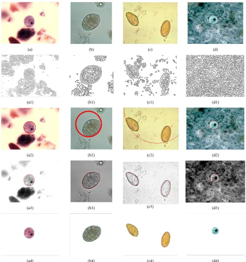
Figure 1 shows the bloc diagram of the proposed method and corresponding illustration for each step. The input is original image with trophozoïte of iodamoeba butschlii (Figure 1 (a)). At the first stage, canny edge detector is applied and Figure 1 (b) shows the result. Hough parameter space is shown in Figure 1 (c). The accumulator with highest vote locates and draws the corresponding circle on image as show in Figure 1 (d2). This circle is used as initial LSF as the 3D view is shown in Figure 1 (d1). DRLSE optimize the contour and the final LSF is illustrated in 3D view of Figure 1 (d3). The contour exactly fit the real shape of parasite (Figure 1 (d4)). The parasite is then extracted and result is presented in Figure 1 (e).

Figure 1. Bloc diagram. (a) Original image with trophozoïte of iodamoeba butschlii. (b) The corresponding edge map. (c) Hough space. The initial LSF (d1) view in 3D and the corresponding image (d2). The final LSF (d3) view in 3D and the corresponding image (d4). (e) The corresponding extracted parasite.

2.4.1. Edge Detection

The edge detection had been employed to perform preprocess of segmentation. The edge information is required for the CHT technique. The canny edge detector consists of the image gradient to highlight regions with high spatial derivatives. The algorithm then tracks along these regions and suppresses any pixel that is not at the maximum. The gradient array is now further reduced by hysteresis. Canny edge follows two threshold values. Pixels that magnitude is under the first threshold are made a non–edge and those with the magnitude are over the high threshold are set as part of edge. When the magnitude is between the two thresholds, the point is set to a non–edge unless there is a path from this pixel to another with gradient above the lower threshold value. The algorithm runs in 5 separate steps:

step 1: Smoothing the image to remove noise.

step 2: Computing gradients so that edges occur for it large magnitudes value.

step 3: Suppresses any pixel that is not at the maximum.

step 4: Potential edges are determined by double thresholding.

step 5: Final edges are determined by suppressing all edges that are not connected to local maxima (Edge tracking by hysteresis).

The Canny edge detector clearly represents each shape and allows to distinctly perceiving the one of the parasite despite the noisy structure of microscopic image. This noisy structure is a great challenge to apply Hough transform.

2.4.2. Location of the Parasite Through Circular Hough Transform (CHT)

space using each edge point. The considered edge point is the center of the drawn circle with a radius r. The values in the accumulator are increased every time a circle is drawn with the desired radius over a cell of the accumulator. The coordinates of the center of the circles in the images are the coordinates of the cell with the highest count and corresponding parameters is used to draw the considered circle on image. The following algorithm describes the CHT scheme on edges provided by canny detector:

step 1: Create a 3D Hough accumulator array

step 2: For each edge pixel (point) draw the considered circle with estimate radius r in the parameter space.

step 3: Increment the corresponding cell in the Hough array.

step 4: Collect candidate circles, and then choose the corresponding circles with highest votes.

step 5: Draw the circle with corresponding parameters on image.

The circle draws on image highlight the interesting zone which contains the parasite to be extract is then used as the initial LSF of the DRLSE. One alternative approach based on gradient vector flow analysis has previously been proposed in [2].

2.4.3. Contour Optimization by Distance Regularized Level Set Evolution (DRLSE)

Considering equation (12), we implemented the DRLSE for image according to LSF

φ

(x, y, t). The derivatives

y

φ

∂ ∂

and

∂ ∂

φ

x

ensuing spaces variables are approximated by the central difference. The space steps are fixed:

∆ = ∆ =

x

y

1

. The temporal partial derivative

∂ ∂

φ

t

is approximated by the forward difference. The discrete form of LSF

φ

(x, y, t) is

φ

_{i j}k_, with spatial index (i, j) and temporal index k. Then, the discrete form of level set evolution equation is given by the equation (13):

(

1

)

( )

, , ,

k k k

i j i j

t

L

i j

φ

+

₋

φ

_{∆ =}

φ

(13)

where

L

( )

φ

_{i j}k_, is the numerical approximation of the right part of equation (12). This conduct to equation (14) which is applied to implement numerically DRLSE [24].

( )

1

, , ,

k k k

i j i j

t L

i j

φ

+

₌

φ

_{+ ∆ ⋅}

φ

,

k

∈

N

(14)

The processing time and requiered memory of a level set method is greatly reduced when it is confined to a narrowband around the zero level set.

Figure 2 presents the flow diagram of the implementation of DRLSE narrowband initialize by CHT. A pixel point (i, j) is considered a zero crossing point, if either

φ

i−1,jand

φ

i+1,j

or

φ

i j, −1and

φ

i j, +1are contrary in signs. The collection of all

the zero crossing points is indexed by Z. The narrowband is constructed as

( )

( , ) ,

v v i j Z i j

B

=

U

_∈

N

(15)

where

N

_{i j}( )_,v is a

(2

v

+ ×

1) (2

v

+

1)

square block centered at

the point

( , )

i j

.

v

can be set to be the minimum value (

v

=

1

), thus the narrowband

B

_v is the union of the 3

×

3 surroundings of the zero crossing points. The LSF is update on the narrowband

B

_vk. Iterations are stopped if either the zero crossing points stop varying for consecutive iterations (

max

n

_ci ) or fixed maximum number of iterations (

max

nbrit

) are exceed.

2.4.4. The Extraction of Parasite

As the initial LSF which is a signed distance function on a signed distance band around the zero level, the final Level Set Function had a positive value inside the contour at the zero level and negative values outside as is shown in Figure 1 ((d1) and (d3)). The zero level contour is the intersection between the zero level plan with the final Level Set Function. It accurately fit on the parasite’s boundary and then segments the image in two: the detected parasite and the background. We simply check all the corresponding pixels with the negative values of final LSF and set them at the value 255 (white color). Our proposed method was applied in other to perform results that some are present in this coming section.

3. Experimental Results and Discussion

3.1. Results

Figure 3. Segmentation results with initial LSF outside the parasite. (a), (b), (c), (d) are original images, (a1), (b1), (c1), (d1) are results of edge detection. (a2), (b2), (c2), (d2) images with initial contour from CHT. (a3), (b3), (c3), (d3) respectively the images with final LSF and (a4), (b4), (c4), (d4) the corresponding extracted parasites.

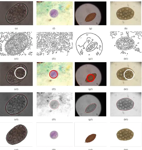
In Figure 4, for original images (e), (f), (g), (h) and their results of edge detection (e1), (f1), (g1), (h1), initial LSF is plot by CHT inside the parasite ((e2), (f2), (g2), (h2)). The weighted area term is set at negative values for the backward diffusion. The corresponding result of final LSF exactly fit with the boundary of parasite is shown at (e3), (f3), (g3), (h3) and their corresponding extracted parasites are respectively

Figure 4. Segmentation results with initial LSF inside the parasite. (e), (f), (g), (h) original images, (e1), (f1), (g1), (h1) are results of edge detection. ((e2), (f2), (g2), (h2)) images with initial contour from CHT. (e3), (f3), (g3), (h3) respectively the images with final LSF and (e4), (f4), (g4), (h4) images with their corresponding extracted parasites.

We present in Figure 5 other results of our algorithm when applied on microscopic images. Figure 5 (o1) to (o10) are originals images with their corresponding extracted parasites in images are respectively presented in Figure 5 (r1) to (r10). The robustness of our algorithm is confirmed in both the

Figure 5. Other results: o1 to o10 are originals images and r1 to r10 their corresponding extracted parasites.

3.2. Discussion

For edge detection, sensitivity high threshold was set to 0.06 and low threshold was 0.4*0.06=0.024. The LSF base coefficient of the distance regularization term

0.2

tstep

µ

=

with time step

tstep

=

5

; the coefficient of the weighted length term

λ

=

5

; These parameters of energy give by equation (9) remain at that standard values. Only the estimated radius for localization by Hough transform and the weighted area term which is used for

forward-and-backward evolution control of Level Set Function. Thus the proposed scheme attempt to be more automated because the number of parameters to be set for segmentation is considerably reduced.

17.636 and 46.466 seconds. Here an appropriate initial level set functions are given so that the result is independent of this initialization (the same results are obtain with (ik1), (ik2), (ik3) and (ik4) initialization) but the scheme underline the region with different intensity without identify the parasite. For DRLSE proposed in [24], initialization (ik1), (ik2), (ik3) and (ik4) is done manually as a rectangle and the parasite can only been clearly detected if they is not other debris near it as shown in result (rk1), (rk2) (rk3) and (rk4) after respective time of 21.891, 4.457, 5.435 and 40.902 seconds. In other words, this method required manual initialization and is

Figure 6. Detection results of our method compared to two other recent methods. (oi1), (oi2), (oi3) and (oi4) are original images; (il1), (il2), (il3) and (il4) are

Initial LSF with the method proposed in [29] and their corresponding results are (rl1), (rl2), (rl3) and (rl4). (ik1), (ik2), (ik3), (ik4) are Initial LSF with the

DRLSE method proposed in [24] and their corresponding results are (rk1), (rk2) (rk3) and (rk4). (ij1) (ij2), (ij3) and (ij4) are Initial LSF with our method and

their corresponding results are (rj1), (rj2), (rj3) and (rj4).

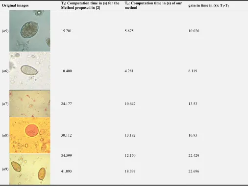
The executing time of our scheme until the real shape detection and extraction of parasite varies between four (4s) and fifteen (50s) seconds depending on the estimate radius and the weighted area term. This executing time should be reduced while using computers with better characteristics than the one used for this work. Our extraction method is less time consuming, less memory required and easier to implement than the one used in [2] where a mask is prior create with the detected contour before make a convolution between the mask and the original image to extract parasites. This is proved by table 1 where we compare the computation time of our method

(T2) to the one of method proposed in [2] (T1). The images (o1) to (o9) are the original images. Example presents in Figure (o9) which presents the highest computation time of our method could not been compare because active contour used in [2] do not allow topology change. But while extract separately each Clonorchis Sinensis our method steel perform best computation time. The third column gives for each case the gain time (T1- T2) while use our method instead of the one presented in [2]. Thus we gain in average 17.5427 for each case. This would significantly increase the number of exam that is realized per days.

Table 1. Scheme computation time comparison. (o1) to (o9) are originals images, T1 the execution time with method proposed in [2], T2 their execution time with our method and T1- T2 arethe gain time.

Original images T1: Computation time in (s) for the

Method proposed in [2]

T2: Computation time in (s) of our

method gain in time in (s): T1-T2

(o1) 15.701 5.675 10.026

(o2) 35.973 10.417 25.556

(o3) 28.316 7.442 20.874

Original images T1: Computation time in (s) for the

Method proposed in [2]

T2: Computation time in (s) of our

method gain in time in (s): T1-T2

(o5) 15.701 5.675 10.026

(o6) 10.400 4.281 6.119

(o7) 24.177 10.647 13.53

(o8) 30.112 13.182 16.93

(o9)

34.599 12.170 22.429

41.093 18.397 22.696

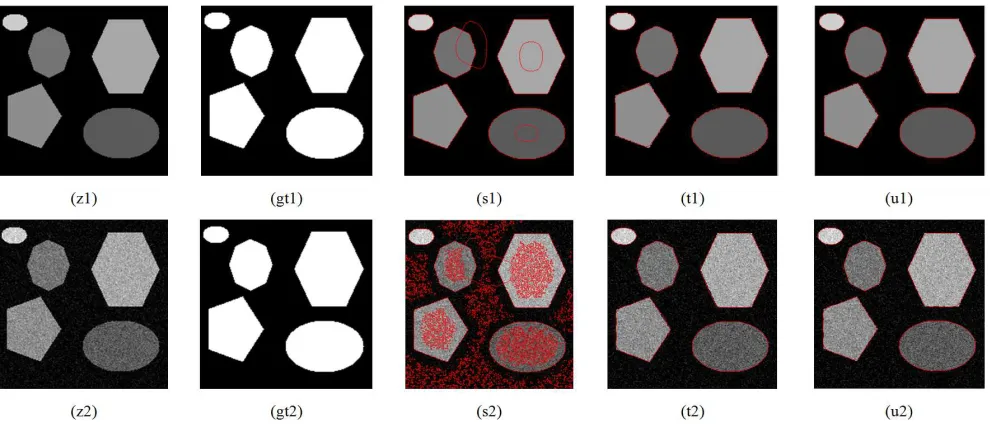
In other to quantitatively evaluate our method, we compare the segmented results of previous different schemes to segmented references images known as ground-truth base on three well known statistical evaluation indexes: misclassification error (ME), the Jaccard distance (JD) and the F-measure. The smaller ME and JD confirm the higher accuracy of the segmentation method, which correspond to the higher F-measure. We denote by tp, tn, fp and fn the true positives, true negatives, false positives, and false negatives respectively for a classifier under test with trusted external judgments. The previous mention statistical evaluation indexes are defined as following:

(

) (

)

ME

=

tp

+

tn

tp

+ +

tn

fp

+

fn

(16)

2.(Re

.

) ( Re

)

F

=

call precision

call

+

precision

(17)

Where

(

)

precision

=

tp tp

+

fp

,

Re

call

=

tp tp

(

+

fn

)

(18)

The Jaccard distance, which measures dissimilarity between the ground-truth foreground object B and the merged segments region A derived from the segmentation

results, is define as:

A B A B JD

A B ∪ − ∩ =

∪ (19)

Figure 7. Quantitative evaluation of segmented results compare to truth. (i1) and (i2) the originals images; (gt1) and (gt2) the corresponding ground-truth images; (s1) and (s2) segmentation results of the method proposed in [29]; (t1) and (t2) the DRLSE segmentation results; (u1) and (u2) segmentation results of the proposed method.

Table 2. Measurement of statistical evaluation indexes of the segmentation. (a) Without noise

method ME JD F

method proposed in [29] 0.0800 0.1978 0.8302 DRLSE 0.0051 0.0143 0.9786 Our method 0.0041 0.0058 0.9992

(b) With noise

method ME JD F

method proposed in [29] 0.7255 0.9696 0.2589 DRLSE 0.0593 0.0154 0.9729 Our method 0.0057 0.0149 0.9891

4. Conclusion

We have proposed in this work a novel method for microscopic image segmentation based on DRLSE automatically initialized using circular Hough transform. The initial level set function is a circle draw around the parasite by circular Hough transform. This initial contour evolves under minimization of energy control until fit the real shape of parasite. A complementary extraction method for the scheme is also proposed. The proposed scheme was applied on a data base of 210 microscopic images with various kind of parasite. Presented results show how accurate and less time consuming the method is. We also qualitatively and quantitatively compared our method to others recent segmentation methods and results approve our method as the best. This represents a significant contribution to the automation of the diagnosis of the intestinal human diseases. The extracted parasite will constitute the training dataset for an algorithm of the automatic recognition of parasite in microscopic images. The method can be extending to magnetic resonance imaging images for the detection of tumor or cancer in tissue such as brain or breast.

Formatting of Funding Sources

This research did not receive any specific grant from funding agencies in the public, commercial, or not-for-profit sectors.

References

[1] Levy L. E., handbook of basic techniques for the medical laboratory, WHO (1999). Vol 1 (912p) & Vol 2 (1000p). [2] Saha T. B., Tchiotsop D., Tchinda R., Kenne G., Automated

Extraction of the Intestinal Parasite in the Microscopic Images Using Active Contours and the Hough Transform, Current Medical Imaging Reviews, Vol. 11, No. 4, pp. 233-246, 2015.

[3] Tchiotsop D., Saha T. B., Tchinda R., Kenne G., Edge detection of intestinal parasites in stool microscopic images using multi-scale wavelet transform, Springer-Verlag London SIViP, vol 9 (Suppl 1), pp. 121–134, 2015. DOI 10.1007/s11760-014-0716-6.

[4] Lecellier F., Jehan-Besson S., Fadili F., Statistical region-based active contours for segmentation: An overview, IRBM (2014), http://dx.doi.org/10.1016/j.irbm.2013.12.002, In press. [5] Fowlkes C., Martin D. and Malik J., Learning to detect natural image boundaries using local brightness, color and texture cues., IEEE Transactions on Pattern Analysis and Machine Intelligence, vol. 26, no. 1, 2004.

[6] Chickanosky V. and Mirchandani G., Wreath products for edge detection, in Proceedings. IEEE International Conference on Acoustics, Speech and Signal Processing (ICASSP), USA, pp. 2953-2956, 1998.

[8] Ying-Don Q., Cheng-Song C., San-Ben C., and Jin-Quan L., A fast sub pixel edge detection method using Sobel-Zernike moments operator., Image and Vision Computing, vol. 23, no. 1, pp. 11–17, 2005.

[9] J. Canny., A computational approach to edge detection, IEEE Trans. Pattern Anal. and Mach. Intell., vol. 8, pp. 679-714, Nov. 1986.

[10] Juneja M., Sandhu P. S., Performance evaluation of edge detection techniques for images in spatial domain., Internationnal Journal of Computer Theory and Engineering 2009; December 2009, pp. 614-621.

[11] Mokate U. B. and Kasturi R., An Algorithm for Recognition of Circles in Graphics., Computer Engineering Technical Report TR-88-061, the Pennsylvania State University, University Park, Pennsylvania 16802, 1988.

[12] Amir I., Algorithm for Finding the Center of Circular Fiducials., Computer Vision, Graphics and Image Processing, 1990. pp 398–406.

[13] Hough P. V. C., Methods and Means for Recognizing Complex Patterns., U.S. Patent vol. 3, 1962 pp 654-669. [14] Duda R. O. and Hart P. E., Use of Hough transform to detect

lines and curves in pictures, ACM Community Management, vol. 15, pp 11–15, 1972.

[15] Ballard D. H., Generalizing the Hough Transform to detect arbitrary shapes, Pattern Recognition vol. 13, 1981, pp 111– 122

[16] Davies E. R., A modified Hough scheme for general circle location, Pattern Recognition Lett. Vol. 7, 1988, pp 37–43. [17] Ho C. T. and Chen L. H., A fast ellipse/circle detector using

geometric symmetry, Pattern Recognition vol. 28, 1995, pp 117–124.

[18] Ho C. T. and Chen L. H., A high-speed algorithm for elliptical object detection, IEEE Transactions on Image Processing, vol. 5 No. 3, 1996, pp 547–550.

[19] Ioannou D., Huda W. and Laine A. F., Circle recognition through a 2D Hough transform and radius histogramming, Image Vision Computer, vol. 17, 1999, pp 15–26.

[20] Olson C. F., Constrained Hough transforms for curve detection, Computer Vision Image Understanding Vol. 73, No. 3, March 1999, pp 329–345.

[21] Osher S. and Sethian J. A., Fronts propagating with curvature dependent speed: Algorithms based on Hamilton-jacobi formulations. Journal of Computational Physics, vol. 79, 1988, pp 12-49.

[22] Sethian J., Level Set Methods and Fast Marching Methods., Cambridge University Press, 1999, book.

[23] Osher S. and Fedkiw R., Level Set Methods and Dynamic Implicit Surfaces., Springer-Verlag New York, Applied Mathematical Sciences, 153, 2002, book

[24] Li C, Xu C, Gui C, Fox M. D., Distance regularized level set evolution and its application to image segmentation. IEEE Transaction on Image Processing, 2010, Vol 19, No: 12, pp 3243-3254.

[25] Yang F, Qin W, Xie Y, Wen T and Gu J., A shape-optimized framework for kidney segmentation in ultrasound images using NLTV denoising and DRLSE., Biomedical Engineering Online (2012) DOI: 10.1186/1475-925X-11-82

[26] Sussman M., Smereka P. and Osher S., A level set approach for computing solutions to incompressible two-phase flow, Journal of Computer Physics, vol. 114, no. 1, Sep. 1994, pp 146–159.

[27] Pochet C. (1), «Parasites des aliments», available on line on

Internet site:

http://bioimage.free.fr/par_image/parasites_aliments.htm. (Date of access: 08.11.2016, 12h30).

[28] Pochet C. (3), « Plan d’étude des formes végétatives et kystiques des protozoaires », available on line on Internet site: http://bioimage.free.fr/par_image/etudeproto.pdf. (Date of access: 08.11.2016, 13h40: 08.11.2016, 15h50).

[29] Li C., Kao C., Gore J. C., and Ding Z., Minimization of region-scalable fitting energy for image segmentation, IEEE Transaction on Image Process., vol. 17, no. 10, Oct. 2008, pp. 1940–949.

[30] Nkamgang OT, Tchiotsop D, Tchinda BS, Fotsin HB, A neuro-fuzzy system for automated detection and classification of human intestinal parasites, Informatics in Medicine

Unlocked (2018), doi:

https://doi.org/10.1016/j.imu.2018.10.007.

[31] Nkamgang OT, Tchiotsop D, Fotsin HB, Talla PK, Louis Dorr Valérie, Wolf D, Automating the clinical stools exam using image processing integrated in an expert system, Informatics

in Medicine Unlocked (2019), doi: