RESEARCHARTICLE
Parameter-free aggregation of value
functions from multiple experts and
uncertainty assessment in
multi-criteria evaluation
Beni Rohrbach
1, Robert Weibel
1, and Patrick Laube
21Department of Geography, University of Zurich, Switzerland
2Geoinformatics Research Group, Zurich University of Applied Sciences, Switzerland
Received: July 14, 2017; returned: October 22, 2017; revised: February 16, 2018; accepted: April 24, 2018.
Abstract: This paper makes a threefold contribution to spatial multi-criteria evaluation
(MCE): firstly by presenting a new method concerning value functions, secondly by com-paring different approaches to assess the uncertainty of a MCE outcome, and thirdly by pre-senting a case-study on land-use change. Even though MCE is a well-known methodology in GIScience, there is a lack of practicable approaches to incorporate the potentially diverse views of multiple experts in defining and standardizing the values used to implement input criteria. We propose a new method that allows generating and aggregating non-monotonic value functions, integrating the views of multiple experts. The new approach only requires the experts to provide up to four values, making it easy to be included in questionnaires. We applied the proposed method in a case study that uses MCE to assess the potential of future loss of vineyards in a wine-growing area in Switzerland, involving 13 experts from research, consultancy, government, and practice. To assess the uncertainty of the outcome three different approaches were used: firstly, a complete Monte Carlo simulation with the bootstrapped inputs, secondly a one-factor-at-a-time variation, and thirdly bootstrapping of the 13 inputs with subsequent analytical error propagation. The complete Monte Carlo simulation has shown the most detailed distribution of the uncertainty. However, all three methods indicate a general trend of areas with lower likelihood of future cultivation to show a higher degree of relative uncertainty.
Keywords:multi-criteria evaluation, land use change, value functions, sensitivity analysis,
1
Introduction
Multi-criteria evaluation (MCE) is a standard methodology in the context of GIScience, with many applications, including the evaluation of potential future land use change. De-spite the ubiquitous use of MCE, however, there is a lack of approaches that allow inte-grating the views of multiple experts in defining the input criteria values, and that are both straightforward to use and transparent regarding the uncertainty that is generated in the MCE.
In this paper, we propose a new, easy-to-use method that enables the integration of the judgments of multiple experts into aggregate, non-monotonic value functions; further, we show how the uncertainty of the MCE outcomes can be assessed. We apply our method to a case study using MCE with multiple experts forecasting the extent of vineyards in a wine-growing area in Switzerland. Within the study area, the extent of vineyards declined by about4%within the past decade and continues to decline. This land use change has implications for landscape beauty, the economic structure of the region as well as the social cohesion [3, 10, 26]. At the same time, this development allows the conversion of areas formerly used as vineyards to other uses, such as biodiversity conservation areas, poten-tially adding ecological corridors between habitats formerly separated by vineyards. Policy makers require predictions of the land use change with a high spatial resolution, in order to proactively react to the current development.
In summary, the paper makes three contributions, two methodological contributions and an applied one. First, we make a contribution to MCE, by introducing a new, simple and parameter-free method to elicit and combine value functions from multiple experts. Value functions are at the core of an important step within any MCE, which until present only few methods tackle. Second, we present a procedure to systematically assess the un-certainty in an MCE, comparing three methods for this purpose: a) one-factor-at-a-time variation, b) a simplified error propagation formula, and c) Monte Carlo simulation. Our results give guidance for further studies to better choose and discuss the results of their sen-sitivity analysis. Third, we make a contribution concerning our case study, the assessment of the suitability for wine-growing within the study area. In the context of this particular paper, the third contribution is of lesser importance and primarily serves to demonstrate the methodological contributions.
1.1
MCE methodology
MCE traditionally comprises six steps [32], as outlined below. Since this manuscript makes methodological contributions to Steps 2 and 5, for the paragraphs concerning those steps a more detailed review of the latest related work is given and the particular research gaps relevant for this paper are specifically highlighted.
Step 1: Selecting criteria. This step typically considers the literature and experts to elicit
the relevant criteria and the values defining them [27, 38].
Step 2: Standardization. Subsequently, one needs to translate the measured values to a
comparable unit (e.g., monetary units or a dimensionless utility) in a comparable range (often 0 to 1) [55]. There are various ways of doing so, mostly by applying a transforming function, e.g., by reclassifying classes of measured values into utility values or by applying a continuous value function [1,2]. The simplest, but ill-advised, way would be to distribute the standardized scores (i.e. 0 to 1) within the range of criteria values [9, 56].
For estimating a value function, the bi-section technique is a prominent representative. Through this approach, one is asked to indicate the level of a measured value that corre-sponds to half of the utility, then with the level of 0.25 and 0.75 utility and finally the level of highest and lowest utility. The intermediate values then are linearly interpolated [22]. However, for the bi-section technique, the functions must be monotonic (i.e., continuously de- or increasing value with increasing input number) [55]. Other approaches yield differ-ently shaped value functions [25], e.g., trapezoidal [35, p.243] or fuzzy membership [11] functions.
Aggregating value functions from the inputs of several participants is difficult, and further advances in group MCE methods are still to be accomplished [33]. Morgan [35] presented an iterative, Delphi-like 6-step procedure to calculate value functions with sev-eral experts. In the published literature, the value functions are chosen ad-hoc [36], com-bined with the weighting step [20], based on a single expert’s opinion [5], or done in work-shops [38]. However, to the best of our knowledge, there is no study presenting a method to elicit and aggregate non-monotonic value functions.
3: Weighting the value scores. One of the more traceable, hence transparent and
con-sequently widespread, weighting methods is the Analytic Hierarchy Process (AHP) [31]. Recent studies have developed new scales for such comparisons, which are more robust concerning inconsistencies and better correspond to verbal expressions [12, 46, 48].
4: Aggregating value scores. This step aims at aggregating the weighted value scores.
There are various different ways of aggregating the criteria, amongst them the Boolean Overlay, Weighted Linear Combination (WLC) and Ordered Weighted Averaging (OWA) methods [57]. Recent studies have complemented the classic aggregation toolbox with more elaborate and complex approaches involving fuzzy aggregation [32, p.231-232], logic scoring of preference [8], and Dempster-Shafer combination [7]. In the case of the WLC, the weighted and standardized criteria are added by summation, which is the most common way of achieving aggregation [32].
5: Sensitivity analysis. Most studies completely neglect to assess the sensitivity of the
time [33], such as by setting the value of a criterion to 0 or to 1. This follows the reasoning “what would have happened, if the measurement or the weighting of this criterion would be completely different.” Such an approach does not consider any possible interactions between criteria, their value functions, and their weightings [29].
The more sophisticated methods focus on assessing sensitivity by including the varia-tion of all the criteria simultaneously, such as analytical calculavaria-tion and probabilistic ods [32, 33]. The probabilistic approach uses Monte Carlo simulation [14] or similar meth-ods, such as bootstrapping [33]. Due to the greater versatility and the less constraining assumptions, Monte Carlo methods today have become the predominant approach to sen-sitivity assessments.
The analytical calculations are based on the formulae for error propagation from gen-eral error theory, according to which the total uncertainty is a combination of the uncertain-ties associated with the individual variable (expressed by the standard deviations of each variable). For reasons of simplicity, the covariance between the criteria often is neglected, which can lead to wrong conclusions. If, for example, high values of one criterion correlate with the low values of another, they compensate each other. If this happens systematically, i.e., if the criteria have a high covariance, the formula yields a higher variation than there actually is. Additionally, general error theory assumes errors to be normally distributed, with the variables being continuously differentiable [32].
In light of practical applications, there is a lack of empirical evidence delivered by stud-ies comparing different methods of uncertainty propagation in MCE. Thus, within this study, we compare the “one-factor-at-a-time” approach, as well as the analytical approach and a Monte Carlo method of assessing uncertainties. Thereof, the “one-factor-at-a-time” could be considered the simplest, and the Monte Carlo approach the computationally most demanding approach.
6: Validation of the results: The validity of the results may be assessed for example in
a stakeholder workshop, through interviews or by means of a questionnaire [27]. As this article focuses mainly on methodological contributions, the validation of the results is pub-lished in [42].
1.2
Related applications of MCEs
MCEs are well suited to land use predictions [54]. Schneider and Pontius [47], for example, calculate the likelihood of deforestation with a spatially explicit MCE. The quality of the predictions by such models varies, however [40]. Additionally, from a policy perspective, land use models should be simple and consider the perspectives of many stakeholders, as this would increase the overall acceptance associated with quantitative models [49].
France
Germany
Italy Switzerland
0 0.5 1 2Kilometers Forest Vineyards River Area of investigation
Source: © swisstopo
Figure 1: Vineyards in the study area in the year 2013. Source: Background hillshading, forests, and vineyards cSwisstopo.
none of the above studies on viticulture followed an explicit procedure to assess the value functions, and none of the studies included a sensitivity analysis.
2
Methods
2.1
Study area
Our case study focuses on the region of Pfyn-Finges, a regional park in the Swiss part of the Rhône Valley, as illustrated in Figure 1. The area is mostly covered by forests (43%), unproductive land (27%), meadows (18%), and built-up areas (6%). Vineyards (4%) and the arable farming (3%) cover for the remaining land [52]. However, visually the vineyards are very prominent, as shown inFehler! Verweisquelle konnte nicht gefunden werden., and they have been a major source of income over a long period of time [3]. Since 2010, the area devoted to vineyards in the region of Pfyn-Finges declined from over 410ha (4.1km2) in the year 2006 to less than 396ha in the year 2014.
2.2
Criteria selection and sampling
Criteria were selected based on a literature review and interviews with three key experts. After discussions with two wine-growers and a first literature review, we selected an initial list of 10 criteria. After two meetings with a key stakeholder and further literature research, we were able to specify the most influential factors more precisely and arranged 9 criteria in a hierarchical tree with the top objective being “Most likely a vineyard in 25 years” (the period of 25 years was chosen as it reflects the average life expectancy of vines in commercial wine-growing).
mod-ified in the first two expert interviews, and then stayed the same for the remaining 11 interviews (n=13). The result is displayed in Figure 5.
2.3
Value functions
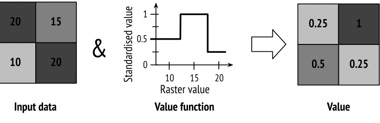
We standardized the criteria values by using so-called value functions [16, 32], which re-classify the criteria-layers values to values on a normalized scale, ranging 0–1. Figure 2 illustrates the normalization of a 4-pixel raster. The resulting value corresponds to the prob-ability that this pixel will be a vineyard in 25 years based on this criterion. Therefore, the value function may vary according to the decision-maker [1,25], as well as in space [16,32]. In our case, there were no indications of varying value functions over space.
20
20
15
10
&
0.25
0.25
1
0.5
Value
Input data
Value function
1
0.5
0
20 15 10
Raster value
Standardised
value
Figure 2: Standardization of the input data of one criterion. The figure uses an arbitrary 4-pixel raster and an arbitrary simple value function, which is used to normalize the raster cell values. Darker cells correspond to higher values.
Through interactions with the experts, we have come to realize that they talked in ranges of optimal values and thresholds for values consider too high or too low, respec-tively, similar to the value functions shown in Morgan [35, p. 243] and similar to the rough set theory [39]. This did not seem to be particular to the subject of wine-growing. In order to adjust the method to the experts’ way of reasoning, we introduced these categories in our survey and propose to do so in other surveys too.
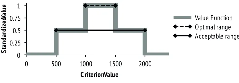
Based on the ranges given by the experts, we calculated classes of input (criterion) val-ues that yield equal standardized valval-ues. The standardized value for a criterion value was calculated according to the number of experts stating that this criterion value lies within the optimal and/or the acceptable range. Figure 3 shows the value function for a single expert for an arbitrary criterion. One could think of, for example, altitude, and then under-stand the criterion values (horizontal axis) as meters. However, we intentionally left the unit dimensionless, as this illustration should only serve as an example.
0
0.25
0.5
0.75
1
0
500
1000
1500
2000
Standardized
Value
Criterion Value
Value Function
Optimal range
Acceptable range
Figure 3: Value function for one criterion and a single expert. The four values provided by the expert are indicated with a black diamond.
(i.e. between 500 and 1000, or 1500 and 2000), it is given a standardized value of 0.5. If the criterion value falls outside both ranges, it receives a value of 0.
In our survey, we asked the experts to indicate the optimal range, the upper and the lower limit for each criterion. If the experts left out an upper or lower limit, we discussed the value and set the value to either zero or positive/negative infinity. For example, the “distance to the road” of a parcel cannot be too small, so the lower limit is given naturally (0m), while there still is an optimal and an acceptable upper limit (visible in Figure 7).
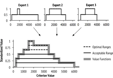
When taking several experts together, we propose the following procedure, as shown exemplarily in Figure 4 for three experts. In the example, all three experts denoted criterion values between 1500 and 2000 as optimal range. Two of the three experts considered values up to 3500 to be optimal, whereof one expert classified values from 1000 on as optimal. Our new method now calculates the standardized value out of the share of overlapping accept-able and optimal ranges given by the experts. For instance, in the illustration, there are three experts with a maximum of 6 ranges overlapping (3 optimal + 3 acceptable ranges). If all optimal ranges overlap (i.e. between the criteria value 1500 to 2000), the standardized value will be 1 (6 of 6). If two of three optimal ranges overlap (plus the three acceptable ranges), the standardized value is 0.83 (5 of 6). If there are only acceptable ranges over-lapping, the standardized value equals 0.5 (3 of 6) and if there is only one expert stating the criterion value to be acceptable its standardized value is 0.16 (1 of 6). The resulting value function resembles very much a fuzzy membership function as, for instance, in [11]. However, the continuous curves in popular fuzzy membership functions are difficult to im-plement and are much more demanding concerning computing power, as opposed to the simple reclassify functions available in standard GIS raster analysis, while yielding only minor differences in practice.
!"
!#$%"
!#%"
!#&%"
'"
!"
'!!!"
$!!!"
(!!!"
)!!!"
%!!!"
*!!!"
!"#$%#&%'()%*
+
#,-)*
.&'")&'/$*+#,-)*
+,,-./012-"3045-6"
7028-"984,/:;46"
<./:=02"3045-6"
0
2000
4000
6000
Expert 2
0
2000
4000
6000
Expert 3
0
0.5
1
0
2000
4000
6000
Expert 1
Figure 4: Value function for one criterion, as a result of the opinions of three experts. The three experts each provide a range for optimal and acceptable values, which then are com-bined by “stacking” them on top of each other.
2.4
Criteria weights
For our case study, we weighted the criteria according to the analytical hierarchy process (AHP) [45]. The participants performed pairwise comparisons on a diverging 9-point scale, ranging from one criterion dominating over another criterion to the other criterion being dominant, with both criteria equally important in the middle. Instead of using a ratio scale, as originally proposed [45], the balanced scale was used as it proved to better reflect people’s judgments and is more robust in the presence of inconsistencies [12,46]. In order to aggregate the individual weights matrix to a group weights matrix, we used the geometric mean as proposed in the literature [18]. We then calculated the criteria weights from the matrix using the “AHP” function in the R package “pmr” [28]. This yielded the weight of each criterion. The weighted values were then aggregated by linear summation.
2.5
MCE sensitivity analysis
method, which is well-known in terms of its abilities to estimate standard deviations [6,15]. The bootstrapping draws random samples of equal size from the total data with replace-ment. In our case, this means the random selection of several groups of 13 participants out of the total 13 participants, wherein some participants may occur several times. After analysing several runs and bootstrap sizes, we concluded that the Standard Deviation (SD) stabilized well before 500 bootstraps. As a summary, we performed the following three procedures to calculate the total uncertainty.
Complete Monte-Carlo simulation: In this procedure, we bootstrapped 500
representa-tions of the sample and accordingly calculated the outcome of the MCE for each bootstrapped resample. We then calculated the SD per pixel out of the 500 runs. This approach includes all interaction effects, but is computationally demanding, as it requires to perform for each pixel 500 MCE runs (one per bootstrap) and to calculate the SD out of the 500 runs.
Analytical combination of the SD per criterion: We took the 500 bootstraps and
calcu-lated the SD per input value for each criterion, as shown as dashed line in the results (Figure 7). The SD per input value was used to reclass the spatial data, resulting in a spatial layer of SD per criterion. This spatial layer then was multiplied with the SD of the criterion’s weight. We then aggregated the SD analytically per pixel by using the following error propagation formula: V artot = PV arcriteria, as suggested in
Malczewski [32, p. 270]. This approach does not include interaction effects between criteria, but has the advantage of being computationally less demanding, as there are fewer operations to be performed per pixel. That is, one reclassification per criterion plus one summation.
“One-factor-at-a-time” variation: For this approach, the weight of a single criterion was
set to 0 and in a second round to 1. The weights of all criteria were then normalized to again sum up to 1, with the value function staying the same throughout the process. As a consequence, two MCE runs were performed per criterion, resulting in a total of 18 runs. Then, the SD per pixel out of the 18 runs was calculated. This procedure is simple and computationally not demanding.
3
Results
3.1
Criteria selection
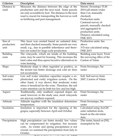
Criterion Description Data source Distance to
road
Measures the distance between the edge of the production unit and the next road. Some parcels are only accessible by foot. The distance to the next road is crucial for transporting the harvest as well as fertilizing and pest management.
Streets: Swisstopo TLM 2014 (all streets wider than 2 m, manually checked).
Production units: Cantonal survey of parcels, manually checked and aggregated to production units. Distance calculated using FME 2015.
Size of production unit
This layer was created based on cadastral data, and then checked manually. Some parcels are very small, e.g., due to partible inheritance and there-fore not suited for large-scale production.
Production units: See above
3-D size calculated using FME 2015
Building zone
The vineyards, which are inside of the building zone, may be used for housing. This increases the land value and thus opens lucrative alternatives to wine farming.
Building zone layer: From the surveying office of the Canton of Valais
Slope Moderate slope is often regarded as positive, as the terrain has better drainage and cold air does not accumulate.
From Swisstopo, 5m raster
Soil water retention
Low soil water retention capacities require a so-phisticated and costly irrigation system. On the other hand, it was shown that moderate water stress is beneficial for the wine. Therefore, the soil water retention can be both too low and too high.
Soil: Soil survey from 2007, Canton of Valais
Aspect Traditionally, only southern exposed slopes are used; however, in the study area, most vineyards are anyway southern exposed.
From Swisstopo, 5m raster
Altitude Altitude together with the insolation determines temperature.
From Swisstopo, 5m raster
Insolation Insolation is important for the ripening of the grapes, especially between April and October.
Calculated using ArcGIS solar radiation tools, based on the elevation data.
Precipitation High precipitation can foster mould; low values can be compensated by irrigation, but increase costs. As winter and spring precipitation is not crucial, we summed the precipitation from July to October
25m raster, based on [59], resampled to 5m
Table 1: Criteria used within the MCE.
Most likely a vineyard in 25 years
Economic factors Natural factors
Building zone Parcel size
Distance to road
Terrain Climate
Slope Soil water retention Aspect Altitude Insolation Preciptation
67% 33%
37%
40% 23%
37% 35% 28% 38% 35% 27%
63% 37%
7.6%
24.9% 15.4% 7.3% 5.9% 4.7% 4.4% 3.3%
26.5%
Figure 5: Criteria tree with intermediate and final weights. The lowest level of boxes shows the individual criteria, with the final weights written beneath. The numbers on the branches of the tree denote intermediate weights.
3.2
Criteria weights
Figure 5 shows the criteria resulting from the AHP process conducted with the 13 ex-perts. The tree is annotated with intermediate weights on the branches and the final criteria weights underneath each criterion. The criteria are shown in the order of decreasing weight from left to right. “Distance to road” received the biggest weight, whereas “Precipitation” yielded the smallest.
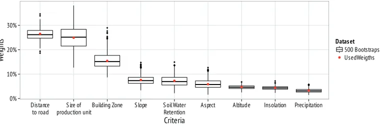
The weights assigned by the 13 experts then were resampled via the bootstrapping method, in order to estimate the variation of each criterion weight. Figure 6 shows the comparison of the aggregated values from all 13 experts with the boxplots of value distri-butions resulting from 500 bootstraps. It becomes clear that the influence of the size of the production unit exhibits the largest variability.
3.3
Criteria value functions
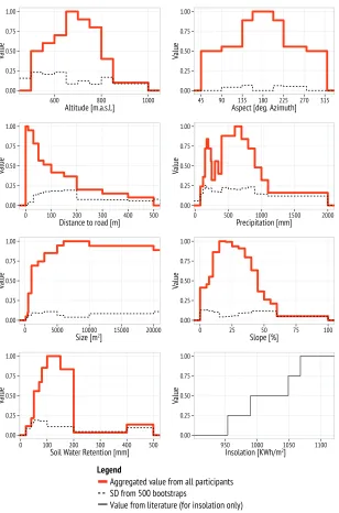
Figure 7 shows the resulting value functions after aggregation. The value functions then are used to standardize the input criteria layers. Figure 8 displays the standardized criteria layers. Figure 7 further displays the standard deviations associated with each criterion value (i.e., vineyards on an altitude of 600ma.s.l. yield a value of 0.7 with an associated standard deviation of nearly 0.25 in respect to altitude). Vineyards that yield values close to 1.00 on all the criteria are very likely to still be cultivated in 25 years from the time of the study.
3.4
Spatially explicit results and associated uncertainty
0% 10% 20% 30%
Distance
to road production unitSize of Building Zone Slope Soil WaterRetention Aspect Altitude Insolation Precipitation
Criteria
W
eights
Dataset
500 Bootstraps Used Weigths
Figure 6: Criteria weights range from 500 bootstraps compared to the weights used. The red points represent the aggregation of all experts and the boxplots the variation over 500 bootstraps.
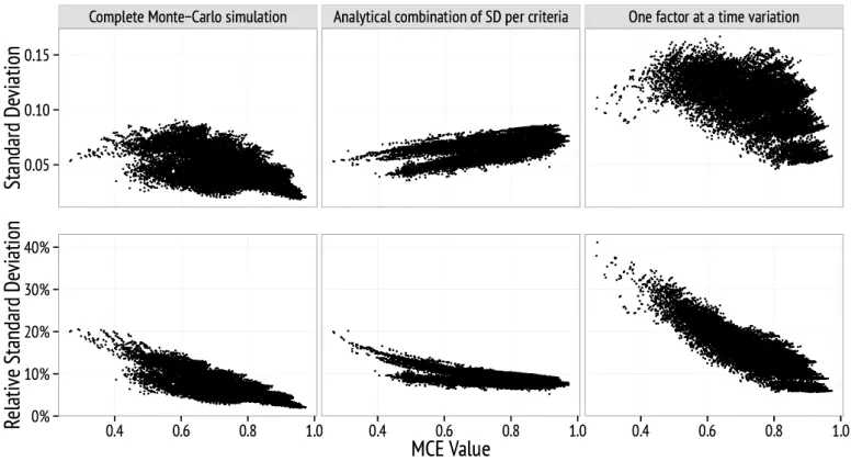
Figure 10 shows the value of the standard deviation (SD) and the relative SD in relation to the MCE outcome and the method of calculation. Each point in the graph corresponds to a pixel of the MCE. The relative SD equals the SD divided by its MCE value. Figure 11 shows the spatial representation of the relative SD. Each pixel in Figure 11 corresponds to a point in Figure 10. Higher values of the relative SD indicate higher uncertainty associ-ated with the outcome. Points to the lower right of Figure 10 correspond to pixels with a high probability of continuing grape production with, at the same time, a low uncertainty attached to this forecast. By contrast, points to the upper left encompass a low likelihood of continuing cultivation, with more uncertainty associated to the prediction. In the case of the complete Monte Carlo simulation, smaller uncertainties indicate a greater level of agreement among the experts.
The mean of the relative SD of the complete Monte Carlo simulation (4.14%, SD = 1.17%) is slightly lower than the one for the analytical combination of the SD per criterion (6.58%, SD=0.77%), with the one from the “one-factor-at-a-time variation” being highest (9.97%, SD = 2.45%). The relative SD from the complete Monte Carlo simulation ranges from 1.9 to 20.6%, with the one based on the analytical combination of the SD ranging from 5.2 to 20.1%. Comparatively, the relative SD from the “one-factor-at-a-time variation” is highest, with a range of 5.7 to 41.2%.
4
Discussion
4.1
Involving a group of experts in a spatial MCE
0.00 0.25 0.50 0.75 1.00
600 800 1000
Altitude [m.a.s.l.] Value 0.00 0.25 0.50 0.75 1.00
45 90 135 180 225 270 315 Aspect [deg. Azimuth]
Value 0.00 0.25 0.50 0.75 1.00
0 100 200 300 400 500 Distance to road [m]
Value 0.00 0.25 0.50 0.75 1.00
0 500 1000 1500 2000 Precipitation [mm] Value 0.00 0.25 0.50 0.75 1.00
0 25 50 75 100
Slope [%] Value 0.00 0.25 0.50 0.75 1.00
950 1000 1050 1100 Insolation [KWh/m2]
Value 0.00 0.25 0.50 0.75 1.00
0 100 200 300 400 500 Soil Water Retention [mm]
Value 0.00 0.25 0.50 0.75 1.00
0 5000 10000 15000 20000
Size [m2]
Value
Legend
Aggregated value from all participants SD from 500 bootstraps
Value from literature (for insolation only)
0 0.5 1 2 Kilometers
Altitude Aspect
Distance to road Precipitation
Size Slope
Soil Water Retention Insolation
Building Zone
Base Elements
Waterways
Outline Vineyards
High : 1
Low : 0 Value of criteria
Elements for orientation Settlements Rivers
0 0.5 1 2
Scale in Kilometers Resulting Score
0.27 0.97
Figure 9: The map shows the results of the MCE, with 1.00 representing the highest proba-bility of continuing grape production. There are few areas with low scores, such as close to the village on the left side of the map.
0 0.5 1 2 Scale in Kilometers Elements for Orientation
Settlements Rivers
Complete Monte-Carlo simulation
Analytical combination of SD per criterion
One factor at a time variation
Relative SD
1.9% 20.6%
Relative SD
5.2% 20.1%
Relative SD
5.7% 41.2%
aversive personality traits, as is included in the bi-section method [24]. However, it could be considered in the proposed procedure in a similar way as in [24].
The aggregation of the value functions among several experts was easily possible. Cur-rent spatial MCE studies aggregate the participants’ value functions through discussions and iterations [35, 38]. By using our methodology, we were able to elicit the value func-tions independently of each other and without interacfunc-tions between the experts, such as, for example, in a delphi-approximation. Hence, this method overcomes the influence of dominant individuals and anchoring biases [43]. It further accounts for minority opinions and different optimal system configurations and therefore allows for alternative optimal configurations.
We assumed values within the acceptable range, but outside the optimal range, to yield a suitability of 0.5, which remains an assumption. As for the bi-section technique, the in-terpolation between the revealed values remains challenging. A possibility would be to generate continuously sloped curves, which, however, would require more complex re-classifying algorithms (and in practice is discretized also in fuzzy membership function evaluation).
Nevertheless, the criteria could be disentangled further in an effort to obtain monotonic functions, as recommended by Winterfeldt and Edwards [55]. The altitude criterion, for instance, could be deconstructed into the maximum altitude for sufficiently high atures (long enough growing season) and the minimum altitude for suitably low temper-atures (not too early ripening). However, whilst this deconstruction may correspond to one expert’s view, another one may perceive different underlying causes for optimal alti-tude. For example, the maximum altitude may as well depend more on the likelihood of serious frosts. Disentangling all the criteria for all possible views would likely render the procedure impracticable due to the thus required extended questionnaire, necessitating additional weighting and valuing. The additional complexity of such a procedure would further blur the comprehensibility and accessibility of the MCE model [13, 34], which is considered an important factor for the trust in the outcomes [19] and further could cause a cognitive overload on the stakeholders [51] that are confronted with the outcome of a thus generated MCE. The MCE method proposed in this study therefore presents a trade-off between scientific credibility and practical suitability.
4.2
Validation of the value functions
In order to validate the plausibility of the elicited and aggregated value functions we com-pare them with comparable values found in the literature (Table 2). We comcom-pare our value functions in the range of 0.5 and higher (“acceptable” to “optimal” values) to the corre-sponding published value ranges.
can be compensated with irrigation, exceedingly high soil water retention capacities cannot be compensated for. Hence, the value function for the soil water retention capacity shows lower optimal values than in the literature. To sum up, the criterion-by-criterion compar-ison with related studies reported in the literature strengthens our trust in the robustness of our proposed approach for aggregating value functions—“robust” meaning that stable results can be produced even with rather diverging individual opinions.
Criterion Value functions of this study Ranges given in the literature
Altitude The elicited value function reaches≥0.5at 500–800m.a.s.l., which is well in line with the literature.
[21]: 400–800m is best [50]: 400–800m is best
Aspect The elicited value function reaches≥ 0.5
at 45–320◦, which is broader than the range found in the literature.
[17]: 135–180◦is best [21]: 135–224◦is best
Distance to road
The value function clearly indicates parcels close to the road to have a higher value.
[41]: The closer the road, the better
Precipitation The bi-modal value function reflects the different cultivation systems used in the study area, either with or without irriga-tion. The temporal distribution of rain over the year was not considered, as it does not differ within the study area.
[20]: Depends on the time of the year and the local conditions
Size The value function shows a trade off be-tween larger parcels and raising capital costs.
This effect was not discussed in the literature yet, to the best of our knowledge.
Slope The elicited value function reaches≥0.5at 7–45%, which starts somewhat lower than reported values, but is very much within the range found in the literature.
[58]: 13–56% is best [17]: 18–33% is best [21]: 11–33% is best [50]: 22–56% is best Soil Water
Retention
The elicited value function reaches≥ 0.5
at 50–200mm, which is close to ranges re-ported in the literature.
[58]: 75–200mm are good [21]: 100–300mm are good
Table 2: Comparison of the value functions of this study with values from the literature.
4.3
Uncertainty analysis: Recommendations
Most likely a vineyard in 25 years
Economic factors Natural factors
Building zone Parcel size
Distance to road
Water availability Ripening
Slope
Aspect Insolation Soil water retention
Preciptation Altitude
Relief
Figure 12: Alternative decision tree, not used in the case study.
consider the use of a complete Monte Carlo simulation more appropriate. Nevertheless, performing uncertainty assessment on a criterion-by-criterion basis (as “one-factor-at-a-time variation” or the analytical approach do) is useful, if spatially explicit uncertainty assessment per model input is sought [29].
Calculating relative standard deviations provides insights in areas that potentially have a high uncertainty associated with them. In our case, the areas of lower MCE value, i.e., the areas that are more likely not to be used as vineyards in the future, showed a higher relative standard deviation. This indicates that there is a greater degree of uncertainty in forecasting areas that likely will not be cultivated as a vineyard than areas that are likely to remain vineyards in the future. This insight was consistent among all three methods of uncertainty assessment.
4.4
Limitations and future work
The different experts might not only have perceived different weights, value ranges and a different selection of decisive factors within the MCE, but also might have structured them differently. Figure 12 provides an example of an alternative decision tree, compared to the one used in our MCE, displayed in Figure 5. The exact designs of the decision tree within the group process will always yield one particular representative amongst a set of valid alternatives. We hold no evidence that the decision tree used here did not represent well the experts’ perceptions, and hence assume it to be valid. However, we felt a need to mention the possibility of alternative decision trees, such as the one shown in Figure 12, to be studied in future research.
and the overall development of the grape prices on the market. Neither, ABM or MCE would per se model that.
5
Conclusion
We have proposed a new method to elicit non-monotonic value functions in spatial MCEs that can be easily combined over several experts. Value functions standardize the criteria values, such as altitude, to a value score from 0 to 1. By asking for four data points—the lower and the higher end of both, the acceptable and the optimal range—this procedure is straightforward to implement and has at the same time proven to deliver robust and stable results. We therefore recommend using this procedure in studies requiring the standard-ization of values elicited from several experts.
We applied the proposed method to the case study of an MCE attempting to forecast potential land use change in vineyard cultivation within the next 25 years. According to our study only few vineyards will disappear. This is in line with the development experienced over the past decade of a decline of vineyards by about 4%. The validity of the elicited value functions was assessed through a comparison to the literature, with which we found a high degree of congruency. The validity of the MCE-outcome is presented in [42].
We assessed the uncertainty of the MCE results by three different methods: (a) a one-factor-at-a-time variation, (b) bootstrapping of the 13 input criteria layers with subsequent analytical error propagation, and (c) a complete Monte Carlo simulation with the boot-strapped inputs. We were able to show that the simplified analytical and the “one-factor-at-a-time variation” approaches fail to accurately reflect the MCE’s uncertainty, with the complete Monte Carlo simulation yielding the most insights. However, all three methods deliver insights, as they indicate a prediction non-continuing wine cultivation to have a higher uncertainty than a prediction of a continuing wine cultivation.
Acknowledgments
We are grateful to Dr. Curdin Derungs (University of Zurich) for his useful discussion concerning the value functions. We would like to further thank all the wine-experts and the wine-growers participating in the research and the administration of the nature park of Pfyn-Finges in shaping the research topic. This work was funded by the University of Zurich, with a supporting grant from the Dr. Joachim de Giacomi Foundation.
References
[1] BEINAT, E.Value functions for environmental management. Environment & management. Kluwer Academic Publishers, Dordrecht, 1997.
[2] BRANS, J.-P.,ANDMARESCHAL, B. PROMETHEE Methods. InMultiple criteria deci-sion analysis: state of the art surveys, J. Figueira, S. Greco, and M. Ehrgott, Eds. Springer, 2005, ch. 5, pp. 163–196.
[4] CARVER, S. Integrating multi-criteria evaluation with geographical information sys-tems. International journal of geographical information systems 5, 3 (1991), 321–339. doi:10.1080/02693799108927858.
[5] CHEN, Y., KHAN, S.,ANDPAYDAR, Z. To retire or expand? A fuzzy GIS-based spatial multi-criteria evaluation framework for irrigated agriculture. Irrigation and Drainage 59(2010), 174–188. doi:10.1002/ird.470.
[6] CHERNICK, M. R. Bootstrap Methods: A Guide for Practitioners and Researchers, 2 ed. Wiley, 2007.
[7] COMBER, A. J. Geographically weighted methods for estimating local surfaces of overall, user and producer accuracies. Remote Sensing Letters 4, 4 (2013), 373–380. doi:10.1080/2150704X.2012.736694.
[8] DUJMOVIC, J., DETRE, G.,ANDDRAGICEVIC, S. Comparison of Multicriteria Meth-ods for Land-use Suitability Assessment. InProc. of the Joint 2009 International Fuzzy Systems Association World Congress and 2009 European Society of Fuzzy Logic and Technol-ogy Conference(2009), IFSA-EUSFLAT, pp. 1404–1409.
[9] EASTMAN, J. R., JIANG, H., AND TOLEDANO, J. Multi-criteria and multi-objective
decision making for land allocation using GIS. InMulticriteria Analysis for Land-Use Management, E. Beinat and P. Nijkamp, Eds., Environment & Management. Springer Netherlands, 1998, ch. 9, pp. 227–251. doi:10.1007/978-94-015-9058-7_13.
[10] EMERY, S. Zukunftsaussichten für die Weinberge auf Terrassen und an Steillagen im Kanton Wallis. Tech. Rep. September, Walliser Landwirtschaftskammer, Conthey, 2001.
[11] FEIZIZADEH, B., SHADMANROODPOSHTI, M., JANKOWSKI, P.,ANDBLASCHKE, T. A GIS-based extended fuzzy multi-criteria evaluation for landslide susceptibility map-ping.Computers & Geosciences 73(2014), 208–221. doi:10.1016/j.cageo.2014.08.001.
[12] FRANEK, J., AND KRESTA, A. Judgment Scales and Consistency Measure in AHP. Procedia Economics and Finance 12, March (2014), 164–173. doi:10.1016/S2212-5671(14)00332-3.
[13] GOLDSTONE, R. L.,ANDJANSSEN, M. A. Computational models of collective behav-ior.Trends in Cognitive Sciences 9, 9 (2005), 424–430. doi:10.1016/j.tics.2005.07.009.
[14] GÓMEZ-DELGADO, M.,ANDTARANTOLA, S. GLOBAL sensitivity analysis, GIS and multi-criteria evaluation for a sustainable planning of a hazardous waste disposal site in Spain. International Journal of Geographical Information Science 20, 4 (2006), 449–466. doi:10.1080/13658810600607709.
[15] GOOD, P. Resampling Methods - A Practical Guide to Data Analysis, 3 ed. Birkhäuser, Boston, Basel, Berlin, 2005.
[17] IRIMIA, L.,ANDPATRICHE, C. Evaluating the ecological suitability of the vineyards, by using Geographic Information Systems (GIS).Cercetˇari Agronomice în Moldova XLIII, 1 (2010).
[18] ISHIZAKA, A., AND LABIB, A. Review of the main developments in the ana-lytic hierarchy process. Expert Systems with Applications 38, 11 (2011), 14336–14345. doi:10.1016/j.eswa.2011.04.143.
[19] JANKOWSKI, P. Towards Participatory Geographic Information Systems for community-based environmental decision making. Journal of environmental manage-ment 90, 6 (2009), 1966–71. doi:10.1016/j.jenvman.2007.08.028.
[20] JONES, G. V., REID, R., AND VILKS, A. Climate, grapes, and wine: Structure and suitability in a variable and changing climate. InThe Geography of Wine: Regions, Terroir and Techniques, P. Dougherty, Ed., vol. 9789400704. Springer, 2012, ch. 7, pp. 109–133. doi:10.1007/978-94-007-0464-0-7.
[21] JONES, G. V., SNEAD, N.,ANDNELSON, P. Geology and wine 8. Modeling viticultural landscapes: A GIS Analysis of the Terroir Potential in the Umpqua Valley of Oregon. Geoscience Canada 31, 4 (2004), 167–178.
[22] KALELKAR, A. S., ANDBROOKS, R. E. Use of multidimensional utility functions in hazardous shipment decisions. Accident Analysis and Prevention 10, 3 (1978), 251–265. doi:10.1016/0001-4575(78)90016-7.
[23] KAYE-BLAKE, W., LI, F., ANDMARTIN, A. Multi-agent Simulation Models in Agri-culture: A Review of Their Construction and Uses. Tech. Rep. 318, Agribusiness and Economics Research Unit, Lincoln University, 2010.
[24] KEENEY, R. L. Value-Focused Thinking. A Path to Creative Decisionmaking. Harvard University School Press, Cambridge, 1992.
[25] KEENEY, R. L., AND RAIFFA, H. Decisions with Multiple Objectives: Preferences and Value Trade-Offs. Cambridge University Press, Cambridge, 1993.
[26] KODER, W. Raron kämpft um seine Rebberge, 2014.
[27] KOWALSKI, K., STAGL, S., MADLENER, R., AND OMANN, I. Sustainable energy futures: Methodological challenges in combining scenarios and participatory multi-criteria analysis. European Journal of Operational Research 197, 3 (2009), 1063–1074. doi:10.1016/j.ejor.2007.12.049.
[28] LEE, P. H., ANDYU, P. L. An R package for analyzing and modeling ranking data. BMC medical research methodology 13, 1 (2013). doi:10.1186/1471-2288-13-65.
[30] LIGTENBERG, A., VAN LAMMEREN, R. J., BREGT, A. K., AND BEULENS, A. J. Validation of an agent-based model for spatial planning: A role-playing ap-proach. Computers, Environment and Urban Systems 34, 5 (2010), 424–434. doi:10.1016/j.compenvurbsys.2010.04.005.
[31] MALCZEWSKI, J.GIS and Multicriteria Decision Analysis. John Wiley & Sons Inc., 1999.
[32] MALCZEWSKI, J. GIS-based multicriteria decision analysis: a survey of the
lit-erature. International Journal of Geographical Information Science 20 (2006), 703–726. doi:10.1080/13658810600661508.
[33] MALCZEWSKI, J.,ANDRINNER, C. Multicriteria Decision Analysis in Geographic Infor-mation. Springer, 2015.
[34] MENDOZA, G.,ANDMARTINS, H. Multi-criteria decision analysis in natural resource management: A critical review of methods and new modelling paradigms. Forest Ecology and Management 230, 1-3 (2006), 1–22. doi:10.1016/j.foreco.2006.03.023.
[35] MORGAN, R. K.Environmental Impact Assessment: A Methodological Approach. Springer Science & Business Media, 1998.
[36] MOSADEGHI, R., WARNKEN, J., TOMLINSON, R., AND MIRFENDERESK, H. Uncer-tainty analysis in the application of multi-criteria decision-making methods in Aus-tralian strategic environmental decisions. Journal of Environmental Planning and Man-agement 56, 8 (2013), 1097–1124. doi:10.1080/09640568.2012.717886.
[37] NEWIG, J., GAUBE, V., BERKHOFF, K., KALDRACK, K., KASTENS, B., LUTZ, J., SCHLUSSMEIER, B., ADENSAM, H., AND HABERL, H. The role of formalisation, participation and context in the success of public involvement mechanisms in re-source management. Systemic Practice and Action Research 21, 6 (2008), 423–441. doi:10.1007/s11213-008-9113-9.
[38] PASSUELLO, A., SCHUHMACHER, M., MARI, M., CADIACH, O., AND NADAL, M. A Spatial Multicriteria Decision Analysis to Manage Sewage Sludge Application on Agricultural Soils. In Environmental Modeling for Sustainable Regional Development, V. Olej, I. Obršálová, and J. Krupka, Eds. IGI Global, 2011, ch. 11, pp. 221–241. doi:10.4018/978-1-60960-156-0.
[39] PAWLAK, Z. Rough Sets.International Journal of Computer and Information Science 11, 5 (1982), 341–356. doi:10.1109/TITB.2009.2017017.
[40] PONTIUS, R. G., BOERSMA, W., CASTELLA, J.-C., CLARKE, K.,DENIJS, T., DIETZEL, C., DUAN, Z., FOTSING, E., GOLDSTEIN, N., KOK, K., KOOMEN, E., LIPPITT, C. D., MCCONNELL, W., MOHDSOOD, A., PIJANOWSKI, B., PITHADIA, S., SWEENEY, S.,
TRUNG, T. N., VELDKAMP, A. T.,ANDVERBURG, P. H. Comparing the input, output,
and validation maps for several models of land change.The Annals of Regional Science 42, 1 (2008), 11–37. doi:10.1007/s00168-007-0138-2.
[42] ROHRBACH, B., LAUBE, P., AND WEIBEL, R. Comparing multi-criteria evaluation and participatory mapping to projecting land use. Landscape and Urban Planning 176 (2018), 38–50. doi:10.1016/j.landurbplan.2018.04.002.
[43] ROWE, G., WRIGHT, G., ANDBOLGER, F. Delphi - A Reevalution of Research and Theory.Technological Forecasting and Social Change 39(1991), 235–251.
[44] RYKIEL, E. J. Testing ecological models: the meaning of validation. Ecological mod-elling, 90 (1996), 229–244.
[45] SAATY, T. L. Decision Making for Leaders: The Analytic Hierarchy Process for Decisions in a Complex World, 3 ed. RWS Publications, Pittsburgh, 1995.
[46] SALO, A. A., AND HÄMÄLÄINEN, R. P. On the measurement of preferences in the analytic hierarchy process. Journal of Multi-Criteria Decision Analysis 6, 6 (1997), 309– 319.
[47] SCHNEIDER, L. C., AND PONTIUS, R. G. Modeling land-use change in the Ipswich
watershed, Massachusetts, USA. Agriculture, Ecosystems and Environment 85(2001), 83–94. doi:10.1016/S0167-8809(01)00189-X.
[48] SIRAJ, S., MIKHAILOV, L., ANDKEANE, J.A. Contribution of individual judgments toward inconsistency in pairwise comparisons.European Journal of Operational Research 242, 2 (2015), 557–567. doi:10.1016/j.ejor.2014.10.024.
[49] SOHL, T. L.,ANDCLAGGETT, P. R. Clarity versus complexity: Land-use modeling as a practical tool for decision-makers. Journal of Environmental Management 129(2013), 235–243. doi:10.1016/j.jenvman.2013.07.027.
[50] STANCHI, S., GODONE, D., BELMONTE, S., FREPPAZ, M., GALLIANI, C., AND
ZANINI, E. Land suitability map for mountain viticulture: A case study in Aosta Val-ley (NW Italy).Journal of Maps 9, 3 (2013), 367–372. doi:10.1080/17445647.2013.785986.
[51] STAUFFACHER, M., FLÜELER, T., KRÜTLI, P., AND SCHOLZ, R. W. Analytic and Dynamic Approach to Collaboration: A Transdisciplinary Case Study on Sustainable Landscape Development in a Swiss Prealpine Region. Systemic Practice and Action Research 21, 6 (2008), 409–422. doi:10.1007/s11213-008-9107-7.
[52] SWISSFEDERALSTATISTICALOFFICE. Landwirtschaftliche Betriebsstrukturerhebung,
2014.
[53] TONIETTO, J., ANDCARBONNEAU, A. A multicriteria climatic classification system for grape-growing regions worldwide. Agricultural and Forest Meteorology 124(2004), 81–97. doi:10.1016/j.agrformet.2003.06.001.
[54] VELDKAMP, A.,ANDLAMBIN, E. Predicting land-use change.Agriculture, Ecosystems & Environment 85, 1-3 (2001), 1–6. doi:10.1016/S0167-8809(01)00199-2.
[55] VON WINTERFELDT, D.,AND EDWARDS, W. Decision analysis and behavioral research, reprint ed. Cambridge University Press, Cambridge, 1986.
[57] YAGER, R. On ordered weighted averaging aggregation operators in multi cri-teria decision making. IEEE Trans. Syst. Man Cybern. 18, 1 (1988), 183–190. doi:10.1109/21.87068.
[58] YAU, I.-H., DAVENPORT, J. R., AND MOYER, M. M. Developing a Wine Grape Site Evaluation Decision Support System for the Inland Pacific Northwestern United States.HortTechnology 24, 1 (2014), 88–98.