http://www.sciencepublishinggroup.com/j/se doi: 10.11648/j.se.20170502.12
ISSN: 2376-8029 (Print); ISSN: 2376-8037 (Online)
Shibuya Method for Computing Ten Knife Edge Diffraction
Loss
Oloyede Adams Opeyemi, Ozuomba Simeon, Constance Kalu
Department of Electrical/Electronic and Computer Engineering, University of Uyo, Akwa Ibom, Nigeria
Email address:
[email protected] (O. Simeon), [email protected] (C. Kalu)
To cite this article:
Oloyede Adams Opeyemi, Ozuomba Simeon, Constance Kalu. Shibuya Method for Computing Ten Knife Edge Diffraction Loss. Software Engineering. Vol. 5, No. 2, 2017, pp. 38-43. doi: 10.11648/j.se.20170502.12
Received: January 3, 2017; Accepted: January 18, 2017; Published: June 7, 2017
Abstract:
Shibuya multiple knife edge diffraction loss method is presented in this paper. The Shibuya method is used to compute the effective diffraction loss of ten multiple knife edge obstructions for a 900 MHz GSM network. Each of the ten obstructions gave rise to a virtual hop which resulted in a knife edge diffraction loss while the overall diffraction loss, according to the Shibuya method is the sum of the diffraction loss computed for each of the ten virtual hops. According to the results, the highest line of sight (LOS) clearance height of 8.480769 m and the highest diffraction parameter of 0.397783 occurred in virtual hop 6. On the other hand, the lowest line of sight (LOS) clearance height of 0.628571 m and the lowest diffraction parameter of 0.044447 occurred in virtual hop 9. Furthermore, the highest virtual hop diffraction loss of 9.30294 dB occurred in virtual hop 6 whereas the lowest virtual hop diffraction loss of 6.38736 dB occurred in virtual hop 9. In all, the overall effective diffraction loss for the 10 knife edge obstructions as computed by the Shibuya is 71.7973 dB.Keywords:
Multiple Knife Edge, Diffraction Loss, Diffraction Parameter, Line of Sight, Clearance Height, Virtual Hop, Shibuya Method1. Introduction
Diffraction phenomenon is described as the apparent bending of waves around obstacles and the spreading out of waves past small openings [1-7]. In respect of the diffraction phenomenon, obstructions in the path of wireless signal cause reduction in the signal strength. This reduction in received signal power due to diffracting obstructions is referred to as diffraction loss [1-11].
The Huygens-Fresnel principle is used to explain the diffraction concept [12, 13]. Particularly, in order to simplify the analysis of diffraction loss, an isolated obstruction like hill or building can be considered as a knife edge obstruction [14-16]. When there are two or more of such knife edge obstructions, then multiple knife edge diffraction loss methods can be employed to determine the effective diffraction loss of all the knife edge obstructions [17]. In this paper, Shibuya method is considered [18], [19]. Like every other multiple knife edge diffraction loss methods, the complexity of the computation increases as the number of knife edge increases. Consequently, most analysis are limited to two or three knife edges. However, in this paper, 10 (ten) knife edge obstructions
are considered and Shibuya method is used to determine the overall diffraction loss that can be caused by the ten knife edge obstruction. The study is conducted for 900 MHz GSM frequency band.
2. Shibuya Multiple Knife Edge
Diffraction Loss Method
Shibuya method relies on the assumption that the ray grazing the obstacles at edge H and H generates a fictitious transmitter E [18], [19]. The procedure for determination of the attenuation due to the diffraction by multiple knife edges is the same as in the Epstein-Peterson method with the difference however that the transmitter E is replaced here by a fictitious transmitter [18], [19].
In figure 1 there are three vitual hop and each virtual hop has one edge that causes diffraction. The three virual hops are;
transmitter for hop 1 whereas E and E are the ficticious or virtual transmitters used in Shibuya diffraction computation for hop 2 and hop 3 respectively. Let the height of the transmitters E , E and E be represented as H , H
and H respetively. Also, from figure 1, it can be seen that, H H . Furthremore, by similar traingle principle, H is given from triangle E H H as follows [18], [19];
Figure 1. None Line –Of Sight Link With Three Obstructions For The Shibuya Method [18], [19].
(1)
H d H d H d H d H d H d (2)
H d H d H d H d (3)
H H (4)
Similarly, h is given from trangle E H H by similar traingle principle as follows; h H H ´ (5)
Where H ´ is the hop 2 line of sight (H To H ) height at a distance of d from the virtual transmitter E at H . H ´ is given by similar traingle as; ´ (6)
H ´ H (7)
h H ! " H (8)
h H H ! " (9)
Similarly, h H H ! # # " (10)
Generally, for any given hop j, the clearance height to its LOS is given as h$where [18]; h$ %H$ H $ & '% ⋯ )&%⋯)*)* )+ &, (11) Where H $ H$ % ⋯ )&%)* ) )* & (12)
A piecewise function is a function that is broken into two or more pieces. The single knife edge diffraction, G$ ./ for each of the virtual hops is computed using Lee’s piecewise knife edge diffraction loss [16, 20-25]. According to Lee’s piecewise model, G$ ./ can be expressed as: G$ ./ 0 11 2 11 3 20log 0.5 0.62v 0 for v$9 1 $ for 1 @ v$ @ 0 20log %0.5exp 0.95v$ & for 0 @ v$ @ 1 20log %0.4 F0.1184 0.38 0.1v$ & for 1 @ v$@ 2.4 20log '. IJ) , for v$K 2.4 L11 M 11 N (13)
Where v$ is the diffraction parameter for virtual hop j. Then, According to the Shibuya multiple diffraction loss
G (dB) = G ./ G ./ ⋯ GO ./ ∑$QO$Q !G$ ./ "(14)
3. Case Study: 10 Knife Edge Diffraction
Loss Computation
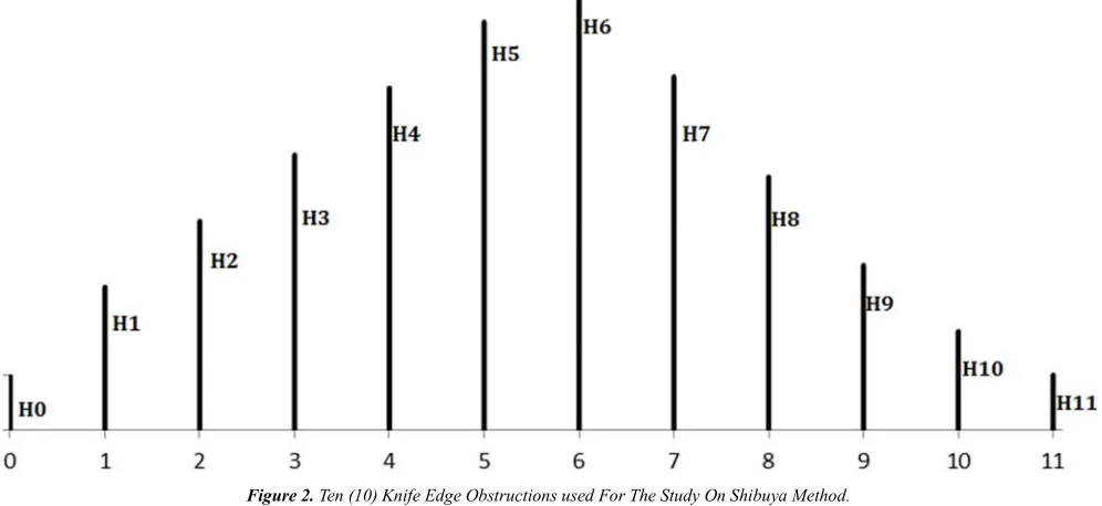
In the case study of figure 2 there are 10 knife edge obstruction with heights H1, H2,…, H10 while H0 and H11
are the transmitter and receiver respectively. Also, the distance of obstruction (i+1) from obstruction (i) is d (i+1) where i= 0, 1, 2,…, 10. The i includes the transmitter with i=0 and the receiver with i=11. Table 1 gives the height, H (i) and the distance d (i) for the 10 knife edge obstructions along with the transmitter and the receiver. The dataset in Table 1 and Figure 2 are used to present numerical computations of 10 knife edge diffraction loss using the Shibuya method.
Figure 2. Ten (10) Knife Edge Obstructions used For The Study On Shibuya Method.
Table 1. The Height Of The Ten (10) Knife Edge Obstructions and the Distance Between Adjacent Obstructions.
Distance (km) Between Adjacent Obstructions Knife Edge Obstruction Height
(Transmitter) H0 10
d1 1 H1 18
d2 2 H2 24
d3 3 H3 30
d4 4 H4 36
d5 5 H5 42
d6 6 H6 45
d7 5 H7 37
d8 4 H8 28
d9 3 H9 20
d10 2 H10 14
d11 1 (Receiver) H11 10
d 36 F =1GHz λ = 0.3
Table 2. The LOS Clearance Height, h (j), The Diffraction Parameter, V (j) and The Diffraction Loss, A (j) For The 10 Virtual Hops As Computed By Shibuya
Method.
j d (j) d (1)+…+d (j) d (j+1) H (j) H (j+) HE (j-1) h (j) V (j) RST UV R
1 1 1 2 18 24 10 3.333333 0.316228 8.62999
2 2 3 3 24 30 15 1.5 0.106066 6.89581
3 3 6 4 30 36 18 1.2 0.070993 6.60641
4 4 10 5 36 42 21 1 0.051962 6.44937
5 5 15 6 42 45 24 3 0.140712 7.1817
6 6 21 5 45 37 34.5 8.480769 0.397783 9.30294
7 5 26 4 37 28 78.6 2.253333 0.117087 6.98675
8 4 30 3 28 20 95.5 1.136364 0.067228 6.57534
9 3 33 2 20 14 108 0.628571 0.044447 6.38736
10 2 35 1 14 10 119 0.972222 0.092233 6.78167
In Shibuya the transmitter E is replaced here by a fictitious transmitter with height H $. Table 2 and figure 3 show that the height H $ of the fictitious transmitter increases with the distance of the obstruction from the anctual transmitter. Also, in the Shibuya multiple knife edge diffraction loss method, each knife edge constitutes a virtual hop with two adjacent knife edge obstructions, or with the transmitter and a knife edge obstruction or with a knife edge obstruction and with the receiver. In this study, the 10 knife edge obstructions gave rise to 10 virtual hops. In Table 2, the results of the LOS clearance height, h (j), the diffraction parameter, V (j) and the diffraction loss, G$ ./ computed for the 10 virtual hops using the Shibuya method are presented for a 900 MHz GSM network. The highest LOS clearance height h (j) =8.480769 m
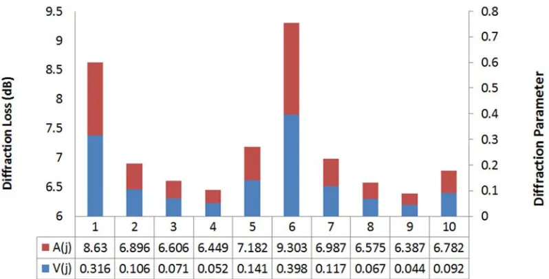
occurred in virtual hop j =6 as shown in Table 2 and figure 3. Also, the highest diffraction parameter, V (j) =0.397783 is obtained in virtual hop j =6, as shown in Table 2 and figure 4. The lowest LOS clearance height h (j) =0.628571 m occurred in virtual hop j = 9. Also, the lowest diffraction parameter, V (j) =0.044447 occurred in virtual hop j = 9.
In Table 2 and figure 5 the lowest absolute value of virtual hop diffraction loss, RG$ ./ R=6.38736dB occurred in virtual hop j = 9 whereas, the highest virtual hop diffraction loss, RG$ ./ R =9.30294dB occurred in virtual hop j =6. In all, the overall effective diffraction loss for the 10 knife edge obstructions as computed by the Shibuya method is 71.7973 dB.
Figure 3. Height W $ of the Fictitious Transmitter and Distance Of The Obstruction From The Anctual Transmitter.
Figure 5. The Diffraction Parameter, V (j) and the Absolute Value Of Diffraction Loss, RX$./ R For The 10 Virtual Hops Of The 10 Knife Edge Obstructions.
4. Conclusions
The application of Shibuya method in the computation of ten multiple knife edge diffraction loss is presented. The study is conducted for a 900 MHz GS|M network. In the computation, each of the ten obstructions gave rise to a virtual hop which resulted in a knife edge diffraction loss. The overall diffraction loss, according to the Shibuya method is the sum of the diffraction loss computed for each of the ten virtual hops. What is peculiar to the Shibuya method is how the virtual hops are identified or defined and the introduction of fictitious transmitters to replace the actual transmitterin each of the virtual hops.
References
[1] Menon, R., & Cantu, P. (2015). U. S. Patent No. 9,063,434. Washington, DC: U. S. Patent and Trademark Office.
[2] Reeves, J., Krinner, L., Stewart, M., Pazmiño, A., & Schneble, D. (2015). Nonadiabatic diffraction of matter waves. Physical Review A, 92 (2), 023628.
[3] Rabiefar, H., Akbarpour, A., & Pourlak, M. (2012). Sensitivity Analysis of Mike21-BW Diffraction Model by using Breakwater Reflection Coefficient.
[4] Sakuyama, T., Funatomi, T., Iiyama, M., & Minoh, M. (2015). Diffraction-Compensating Coded Aperture for Inspection in Manufacturing. IEEE Transactions on Industrial Informatics,
11 (3), 782-789.
[5] Naik, V. (2016). Hyperspectral Radiometer and Ultraviolet Spectrometer Design (Doctoral dissertation).
[6] Wei, Y. (2014, August). Depth reconstruction with Fresnel diffraction. In 2014 IEEE International Conference on Mechatronics and Automation (pp. 61-65). IEEE.
[7] Misra, I. S. (2013). Wireless Communications and Networks: 3G and Beyond. McGraw Hill Education (India) Pvt Ltd.
[8] Wesolowski, H., & Wesolowski, K. (2001). Mobile communication systems. John Wiley & Sons, Inc..
[9] Ghasemi, A., Abedi, A., & Ghasemi, F. (2011). Propagation engineering in wireless communications. Springer Science & Business Media.
[10] Malila, B., Falowo, O., & Ventura, N. (2015, September). Millimeter wave small cell backhaul: An analysis of diffraction loss in NLOS links in urban canyons. In AFRICON, 2015 (pp. 1-5). IEEE.
[11] Phillips, C., Sicker, D., & Grunwald, D. (2013). A survey of wireless path loss prediction and coverage mapping methods.
IEEE Communications Surveys & Tutorials, 15 (1), 255-270. [12] Tyson, R. K. (2014). Fresnel and Fraunhofer diffraction and
wave optics. In Principles and Applications of Fourier Optics. IOP Publishing, Bristol, UK.
[13] Pedrotti, L. S. (2008). Basic physical optics. Fundamentals of Photonics, 152-154.
[14] Östlin, E. (2009). On Radio Wave Propagation Measurements and Modelling for Cellular Mobile Radio Networks.
[15] Baldassaro, P. M. (2001). RF and GIS: Field Strength Prediction for Frequencies between 900 MHz and 28 GHz. [16] Qing, L. (2005). GIS Aided Radio Wave Propagation Modeling
and Analysis (Doctoral dissertation, Virginia Polytechnic Institute and State University).
[17] Barclay, L. W. (2003). Propagation of radiowaves (Vol. 502). Iet.
[18] Sizun, H., & de Fornel, P. (2005). Radio wave propagation for telecommunication applications. Heidelberg: Springer. [19] Shibuya S (1983) A Basic Atlas of Radio-Wave Propagation.
John Wiley & Sons, New York.
[20] Aragon-Zavala, A. (2008). Antennas and propagation for wireless communication systems. John Wiley & Sons. [21] Salous, S. (2013). Radio propagation measurement and
[22] Akkaşlı, C. (2009). Methods for Path loss Prediction. Reports from MSI, School of Mathematics and Systems Engineering, Report, 9067.
[23] Beyer, J. (2004). An approximate approach to predict multiple screen diffraction in the case of grazing incidence. Radio science, 39 (4).
[24] Guo, W., Mias, C., Farsad, N., & Wu, J. L. (2015). Molecular versus electromagnetic wave propagation loss in macro-scale environments. IEEE Transactions on Molecular, Biological and Multi-Scale Communications, 1 (1), 18-25.
![Figure 1. None Line –Of Sight Link With Three Obstructions For The Shibuya Method [18], [19]](https://thumb-us.123doks.com/thumbv2/123dok_us/8489896.1716223/2.595.125.473.131.336/figure-line-sight-link-obstructions-shibuya-method.webp)