A Study on a Tandem Stochastic Queueing Model with Parallel Phases and a Numerical Example

(1)

Published online March 6, 2015 (http://www.sciencepublishinggroup.com/j/sjams) doi: 10.11648/j.sjams.20150302.12

ISSN: 2376-9491 (Print); ISSN: 2376-9513 (Online)

A Study on a Tandem Stochastic Queueing Model with

Parallel Phases and a Numerical Example

Vedat Sağlam

1

, Erdinç Yücesoy

1

, Murat Sağır

1

, Müjgan Zobu

2

1

Department of Statistics, Faculty of Science and Arts, OndokuzMayıs University, Kurupelit, Turkey 2

Department of Statistics, Faculty of Science and Arts, Amasya University, Amasya, Turkey

Email address:

[email protected] (Vedat S.)

To cite this article:

Vedat Sağlam, Erdinç Yücesoy, Murat Sağır, Müjgan Zobu. A Study on a Tandem Stochastic Queueing Model with Parallel Phases and a Numerical Example. Science Journal of Applied Mathematics and Statistics. Vol. 3, No. 2, 2015, pp. 33-38.

doi: 10.11648/j.sjams.20150302.12

Abstract:

In this study a two stage queueing model is analyzed. At first stage there is a single server having exponential service time with parameter and no waiting is allowed in front of this server. There are two parallel phase-type servers at second stage and these parallel servers have exponential service time with parameter . Arrivals to this system is Poisson with parameter . An arriving customer to this system has service if the server at first stage is available or leaves the system if the server is busy where the first loss occurs. After having service in first stage the customer proceeds to the second stage, if both of the phase-type parallel servers in second stage are available the customer chooses one of these servers with probability 0.50 or leaves the system if any of these servers in second stage is busy so the second loss occurs. A customer who has service at both stages leaves the system. The number of customers in this model is represented by a 3-diamensional Markov chain and Kolmogorov differential equations are obtained. After that mean number of customers and mean waiting time in the system is obtained by limit probabilities. We have shown that the customer numbers at first and second stages are dependent to each other. The numerical analysis of obtained performance measures are shown by a numeric example. Finally the graphs of loss probabilities and measure of performances given for some values of arrival rate and the service parameters.

Keywords:

3-diamensional Markov Chain, Tandem Queuing System, Poisson Current, Phase-Type Distributions, Loss Probabilities

1. Introduction

The use of queueing models is essential for studies in telecommunication, computer sciences, production lines, transportation and etc. By modeling queueing systems and analyzing these systems we can optimize the performance measures of such models. In this manner tandem queues and parallel queues are widely studied. One of the important study area in Queueing Theory is the queues with phase-type services which is a common means of obtaining queueing models. In phase-type queues inter arrival and/or service times are phase-type distributed. Many works have done in queueing models. Various possibilities of customer numbers, the mean customer number at every stage and the distribution of waiting time in a tandem queueing system with Poisson stream and with different exponential service time are found in [1]. In a queueing model in which the interarrival times and the service times are general distributed no loss and no

(2)

tandem queueing system with two stages obtained and these performance measures are optimized, the independency of customer numbers at first and second stages is shown and the optimal ordering of service channels are given in [13]. The performance measures of Coxian queueing system are widely analyzed by z-transform and Laplace transform at [14]. Phase-type distributions widely explained in [10]. The generalization to phase-type distributions investigated by [9]. In this paper a two stage queueing system, with a single server at first stage and parallel two phase-type servers at second stage is studied.

2. The Stochastic Queueing Model

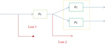
A new two stage tandem queueing model is defined in this paper. In this queuing model arrivals are Poisson with parameter . At first stage there is a single server having exponential service time with parameter and no waiting is allowed in front of this server. There are two parallel phase-type servers at second stage and these parallel servers have exponential service time with parameter . After completing service at first stage a customer chooses one of the parallel servers at second stage with equal probabilities if both servers are available and by completing service at second stage the customer leaves the system. At a same time the parallel servers at second stage both can not serve. If any of two parallel servers at second stage is busy the customer leaves system without having service at second stage, loss occurs.

Figure 1. Stochastic queueing model.

The queueing discipline described above is modeled as following: Let ( ) be the number of customers at first stage,

( ) and ( ) be the number of customers in first server and second server at second stage respectively. We now

define 3-diamensional Markov chain as

( ), ( ), ( ); ≥ 0. The state probability of this chain is denoted by _{, ,} .

, , ( ) = ( ) = , ( ) = , ( ) = (1)

State space of this chain is given as below: ℑ = (0,0,0), (0,0,1), (0,1,0), (1,0,0), (1,1,0), (1,0,1) (2)

where, ∈ 0,1 , ∈ 0,1 , ∈ 0,1.

3. Limit Probabilities

We need to obtain the transient probabilities, for this purpose firstly we obtain Kolmogorov differential equations. Assuming, lim!→# , , ( ) = , , ve lim_!→# ′ _{, ,} ( ) = 0. (3) Kolmogorov differential equations are : %%%&( ) = − %%%( ) + % %( ) + %% ( ) (4)

%% &( ) = −( + ) %% ( ) + 0.5 %%( ) + % ( ) (5) % %&( ) = −( + ) % %( ) + 0.5 %%( ) + %( ) (6) %%&( ) = − %%( ) + %%%( ) + %( ) + % %( ) (7) %&( ) = −( + ) %( ) + % %( ) (8)

% &( ) = −( + ) % ( ) + %% ( ) (9)

And steady-state equations of this Markov chain is obtained as following; 0 = − %%%+ % %+ %% (10)

0 = −( + ) %% + 0.5 %%+ % (11)

0 = −( + ) % %+ 0.5 %%+ % (12)

0 = − %%+ %%%+ %+ % (13)

0 = −( + ) %+ % % (14)

0 = −( + ) % + %% (15)

Transient Probabilities Writing _{, ,} in terms of _%% we get, %%%=₊,_{(+.- .- )}- (- .- )/ %% (16)

% %=%.0- (- .- )_{- (+.- .- )} %% (17)

%% =%.0- (- .- )_{- (+.- .- )} %% (18)

% =_{- (+.- .- )}%.0+- %% (19)

%=_{- (+.- .- )}%.0+- %% (20)

∑ ∑ ∑ , , = 1 (21)

under condition (21), %%=_{, .}2 3.224352 522 / (22)

is obtained. And putting (22) in the equations (16), (17), (18), (19) and (20) the transient probabilities _{, ,} are found as below: %%%= 3 ,2 (2 52 )_{(352 52 )}/ , .2₃.2₂4_{352 52}2 / (23)

(3)

% = %=

6.789 9 (859 59 )

, .9₈.9₉ 4_{859 59}9 / (25)

4. Loss Probabilities

In this queueing model the loss probabilities are defined as

P;<==( ) and P;<==( ) which are the loss at first stage and loss at second stage respectively. First loss P_;<==( ) is calculated as below,

P;<==( ) = %%+ % + %=_+.-+ (26)

This probability depends on parameters and but independent from the parameter . In other words, the loss at first stage is irrelevant to service parameter of second stage. On the other hand second loss, P_;<==( ) can be calculated as given:

P;<==( ) = 1 − > %%%+ %% ?

or,

P;<==( ) = %% + % %+ %+ %

P;<==( ) = @-_- A %%= (μ μ⁄ ) @1 +F D_E +D_D −_{E.D .D}D A (27)

5. Measure of Performances

5.1. Mean Number of Customers in the System

The expected value of G(H) where N denotes the number of customers in the system, is found as follows:

G(H) = ∑ ∑ ∑ ( + + ) , , (28)

G(H) = %% + % %+ %%+ 2( %+ % ) (29)

G(H) = J .9 (859 59 )9 (9 59 ) .9 (859 59 )89

.9₈.9₉ 4_{859 59}9 K (30)

5.2. The Mean Waiting Time in the System

Let T denotes the waiting time of a customer in the system. By the exact expected value formulae we can write following equation:

G(L) = (M)G(L M⁄ ) + (M N)G(L M̅⁄ ) (31) where, the event A represents the loss at second stage.

(M) = P;<==( ) (32)

So, now we can calculate the expected value of G(L) as below:

G(L M⁄ ) =_- (33)

G(L M̅⁄ ) =_- +_- (34)

G(L) =_- + P .2 (352 52 )2 (2 52 )

, .2₃.2₂ 4_{352 52}2 /Q @- A (35)

6. Numerical Example

Now by a simple example the numerical values of P_;<==( ),

P;<==( ), G(H) and G(L) are given in table1, table2, and table3. For some various values of , each situations = 6 and

= 8 , = 8 and = 6, = 7 and = 7 are investigated.

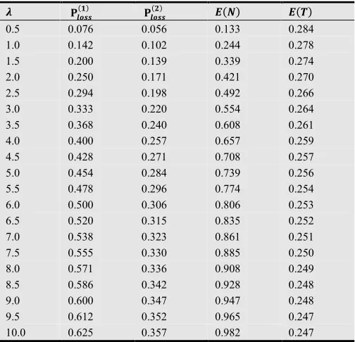
Table 1. Loss probabilities and measure of performances for = 6 and

= 8

U V_WXYY(Z) V_WXYY([) \(]) \(^)

0.5 0.076 0.056 0.133 0.284

1.0 0.142 0.102 0.244 0.278

1.5 0.200 0.139 0.339 0.274

2.0 0.250 0.171 0.421 0.270

2.5 0.294 0.198 0.492 0.266

3.0 0.333 0.220 0.554 0.264

3.5 0.368 0.240 0.608 0.261

4.0 0.400 0.257 0.657 0.259

4.5 0.428 0.271 0.708 0.257

5.0 0.454 0.284 0.739 0.256

5.5 0.478 0.296 0.774 0.254

6.0 0.500 0.306 0.806 0.253

6.5 0.520 0.315 0.835 0.252

7.0 0.538 0.323 0.861 0.251

7.5 0.555 0.330 0.885 0.250

8.0 0.571 0.336 0.908 0.249

8.5 0.586 0.342 0.928 0.248

9.0 0.600 0.347 0.947 0.248

9.5 0.612 0.352 0.965 0.247

10.0 0.625 0.357 0.982 0.247

= 6

U V_WXYY(Z) V_WXYY([) \(]) \(^)

0.5 0.058 0.074 0.133 0.279

1.0 0.111 0.136 0.247 0.268

1.5 0.157 0.186 0.344 0.260

2.0 0.200 0.228 0.428 0.253

2.5 0.238 0.264 0.502 0.247

3.0 0.272 0.294 0.567 0.242

3.5 0.304 0.320 0.624 0.238

4.0 0.333 0.342 0.676 0.234

4.5 0.360 0.362 0.722 0.231

5.0 0.384 0.379 0.764 0.228

5.5 0.407 0.394 0.802 0.225

6.0 0.428 0.408 0.836 0.223

6.5 0.448 0.420 0.868 0.221

7.0 0.466 0.430 0.897 0.219

7.5 0.483 0.440 0.924 0.218

8.0 0.500 0.448 0.948 0.216

8.5 0.515 0.456 0.971 0.215

9.0 0.529 0.463 0.993 0.214

9.5 0.542 0.470 1.013 0.213

(4)

= 7

U V_WXYY(Z) V_WXYY([) \(]) \(^)

0.5 0.066 0.064 0.131 0.276

1.0 0.125 0.117 0.242 0.268

1.5 0.176 0.160 0.337 0.262

2.0 0.222 0.197 0.419 0.257

2.5 0.263 0.228 0.491 0.253

3.0 0.300 0.255 0.555 0.249

3.5 0.333 0.277 0.611 0.246

4.0 0.363 0.297 0.661 0.243

4.5 0.391 0.314 0.706 0.240

5.0 0.416 0.329 0.746 0.238

5.5 0.440 0.343 0.783 0.236

6.0 0.461 0.355 0.816 0.234

U V_WXYY(Z) V_WXYY([) \(]) \(^)

6.5 0.481 0.365 0.847 0.233

7.0 0.500 0.375 0.875 0.232

7.5 0.517 0.383 0.900 0.230

8.0 0.533 0.391 0.924 0.229

8.5 0.548 0.398 0.946 0.228

9.0 0.562 0.404 0.966 0.227

9.5 0.575 0.410 0.985 0.227

10.0 0.588 0.415 1.003 0.226

For some various values the graphs of P_;<==( ), P_;<==( ), G(H),

G(L) are given for each situations < , > and

= . In these graphs the values in tables are used.

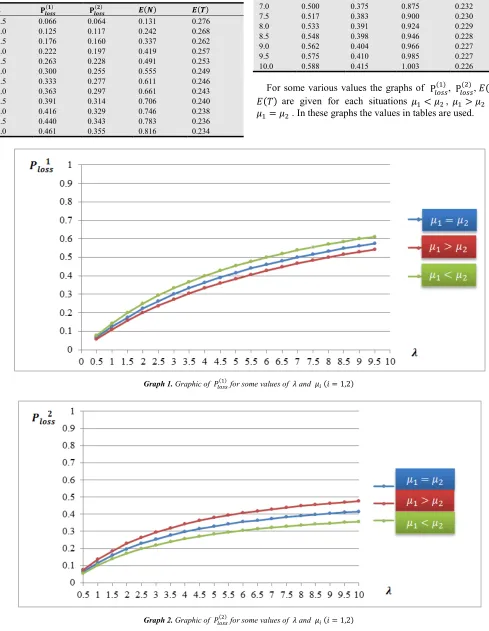
Graph 1. Graphic of _;<==( ) for some values of and _a (b = 1,2)

(5)

Graph 3. Graphic of G(H) for some values of and _a (b = 1,2)

Graph 4. Graphic of G(L) for some values of and _a (b = 1,2)

As we can see in graph1, when the arrival parameter increases the loss probabilities also increase. It is seen in graph2 that when > , the loss probability P_cdee( ) increases according to the other two situations ( < and

= ). And in graph3, even there is no significant difference at G(H) for different _a(b = 1,2) service times, as increases G(H) also increases. Graph2 and graph4 clearly shows that there is a reverse ratio between G(L) and P_cdee( ) .

7. Conclusion

In this paper we have analyzed a two stage, consists of three servers, phase-type stochastic queueing model. The number of customers in the servers at any given t time defined by a 3-diamensional Markov chain. State space is constructed and then Kolomogorov differential equations are obtained. Steady-state equations are found for → ∞ , transient probabilities are obtained by solving the steady-state equations with algebraic methods. After that the loss probabilities at both stages and performance measures are calculated. In the numerical example, for the various values

of arriving rate ( ) and for different and then for the same values of service parameters the corresponding values of

Pcdee( ), Pcdee( ), G(H) and G(L) are given in table1, table2 and table3. Later, for the different values of arriving rate ( ) and for some situations of service parameters the values of loss probabilities P_cdee( ), P_cdee( ) and mean customer numbers in the system G(H), the mean waiting time in the system G(L) is presented by figure1, figure2, figure3 and figure4 respectively. For further studies different queueing models can be constructed by increasing the server number at second stage and these new queueing models can be investigated.

References

[1] Jackson, R. R. P., “Queueing systems with Phase-Typeservice”, Operat. Res. Quart., 5, 109-120, 1954.

(6)

[3] R. K. Rana, “Queueing problems with arrivals in general stream and phase type service” Metrika, vol. 18, no. 1, pp. 69–80, 1972.

[4] V. Ramaswami and M. F. Neuts, “A duality theorem for phase type queues”, The Annals of Probability, Vol.8, No.5, 974-985, 1980.

[5] V. Ramaswami, “Algorithms for the Multi-Server Queue”, Commun. Statist.- Stochastic Models, 1(3), 393-417, 1985. [6] D. D. Selvam and V. Sivasankaran, “A two-phase queueing

system with server vacations”, Operations research letters, Vol.15, no.3, pp.163-169, 1994.

[7] J. R. Artalejo and G. Choudhury, “Steady State Analysis of an M/G/1 Queue with Repeated Attempts and Two-Phase Service”, Quality Technology & Quantative Management, Vol.1, No.2, pp. 189-199, 2004.

[8] B. V. Houdt and A. S. Alfa, “Response time in a tandem queue with blocking, Markovian arrivals and phase-type services”,

Operations Researc Letters 33, pp.373-381, 2005.

[9] Gross, D., Harris, C. M., Thompson, M. J., Shortle, F. J.,

Fundementals of Queueing Theory, 4th ed., John Wiley & Sons, New York, 2008.

[10] Stewart, W.J., Probability, Markov Chains, Queues and Simulation, Princeton University Press, United Kingdom, 2009.

[11] M. Zobu, V. Sağlam, M. Sağır, E. Yücesoy, and T. Zaman, “The Simulation and Minimization of Loss Probability in the Tandem Queueing with Two Heterogeneous Channel” Mathematical Problems in Engineering, vol. 2013, Article ID 529010, 4 pages, 2013. doi:10.1155/2013/529010.

[12] M. Zobu and V.Sağlam, “Control of Traffic Intensity in Hyperexponential and Mixed Erlang Queueing Systems with a Method Based on SPRT” Mathematical Problems in Engineering, vol. 2013, Article ID 241241, 9 pages, 2013. doi:10.1155/2013/241241.

[13] V.Sağlam and M. Zobu, “A Two-Stage Model Queueing with No Waiting Line between Channels”, Mathematical Problems in Engineering, Volume 2013, Article ID 679369, 5 pages. [14] V. Sağlam, M. Uğurlu, E.Yücesoy, M. Zobu, M. Sağır, “On