Design of a Single Stage Centrifugal Compressor as Part of a Microturbine Running at 60000 rpm, Developing a Maximum of 60 kW Electrical Power Output

http://www.sciencepublishinggroup.com/j/ajae doi: 10.11648/j.ajae.20170402.11

ISSN: 2376-4813 (Print); ISSN: 2376-4821 (Online)

Design of a Single Stage Centrifugal Compressor as Part of

a Microturbine Running at 60000 rpm, Developing a

Maximum of 60 kW Electrical Power Output

Munzer Shehadeh Yousef Ebaid

1

, Qusai Zuhair Mohmmad Al-Hamdan

2

1

Mechanical Engineering Department, Faculty of Engineering, Philadelphia University, Amman, Jordan

2_{Aircraft Engineering Department, Perth College, University of the Highlands and Islands, Perth PH2 8PD, Scotland, UK}

Email address:

[email protected] (M. S. Y. Ebaid), [email protected] (Q. Z. M. Al-Hamdan)

To cite this article:

Munzer Shehadeh Yousef Ebaid, Qusai Zuhair Mohmmad Al-Hamdan. Design of a Single Stage Centrifugal Compressor as Part of a Microturbine Running at 60000 rpm, Developing a Maximum of 60 kW Electrical Power Output. American Journal of Aerospace Engineering.

Vol. 4, No. 2, 2017, pp. 6-21. doi: 10.11648/j.ajae.20170402.11

Received: March 6, 2017; Accepted: April 5, 2017; Published: July 20, 2017

Abstract:

In this current work, the design of a single stage centrifugal compressor as part of a complete small gas turbine coupled directly to high speed permanent magnet running at 60000rpm and developing a maximum electrical power of 60kW is presented. The choice of a radial impeller was considered and the design was based on using a non-linear optimisation code to determine the geometric dimensions of the impeller. Also, the optimum axial length and the flow passage of the impeller were found based on prescribed mean stream velocity. The proposed code was verified and showed quite good agreement with the published data in the open literature. The design of a vaneless diffuser and a volute were considered based on satisfying the governing equations of conservation of mass, momentum, and energy conservation simultaneously. Results showed good agreement with the CFD analysis found in the open literature. This work was motivated by the growing interest in micro-gas turbines for electrical power generation, transport and other applications.

Keywords:

Centrifugal Compressor, Vaneless Diffuser, Impeller, Mean Stream Velocity, Optimization

1. Introduction

Centrifugal compressors are one of the main components of microtubines. Microturbines are gas turbines with power ranging approximately from 10 t0 200kW. These devices can be used in stationary, transport and auxiliary power application. In the compressor design stage, many choices of design options need to be considered before the final design. It is essential that design engineers begin to perform a compressor design with full understanding of all aspects of the design considerations [1–4]. Many research works that have been cited in the open literature used different optimization methods such as artificial neural network (ANN) and a genetic algorithm (GA), developed computer codes, and Computational fluid mechanics (CFD) to design the centrifugal impeller. These were based on the design variables that control the shape of the impeller [5-12]. However, the superiority of these design techniques could not be validated in experimental results due to the difficulties in properly

conducting experiments.

2. Design Problems

impeller flow passages. Stahler [14] investigated the effect of inducer relative tip Mach number Mer on efficiency using

several Boeings compressors. The results were presented indicate the penalty that may be paid for the increase inMer.

Efficiency falls off rapidly forMer greater than 0.8.

Third problem is the radial vaneless diffuser which may be considered a major source of inefficiency in centrifugal compressors due to non-uniform flow leaving the impeller; therefore, most of the work cited in the open literature was directed to study the flow and find methods to predict the losses in the vaneless diffuser in an attempt to increase its efficiency, [15-20]. According to this, careful design is addressed to the vaneless diffuser to produce efficient compressor.

Betteni at el. [21] presented the design process for a centrifugal compressor that will be part of demonstrative micro-gas turbine plant. The design methodology developed at Dimset has been used for the fluid dynamics design of a centrifugal compressor for a small micro gas turbine plant. Zahed and Bayomi [22] presented the development of a preliminary design method for centrifugal compressors. The design process started with the aerodynamic design and its reliance on empirical rules limiting the main design parameters. This procedure can be applied to the compressors for the pressure ratios of 1.5, 3.0 and 5.0. Design considerations of mechanical stress for the impeller and minimum inlet Mach number were taken into consideration. In this research work, the authors had done the preliminary design in which the work input and compressor efficiency was considered. The impeller design at different pressure ratios has been done.

Marefat et al. [23] presented the design procedure of multi-stage centrifugal compressor, by considering one dimensional flow design. The design procedure started from calculation of impeller inlet and it is continued for the other sections including impeller exit, diffuser and volute. The total efficiency, stage efficiency, correction factors and leakages are calculated. From the procedure. it was revealed that there are essential parameters such as tip speed Mach number, flow co-efficient at inlet and diameter of impeller which will play major roles in determining compressor polytropic head and consequently compressor polytropic efficiency. The designed volute is different than that the referred one. The dissimilarity rises on the grounds that the mentioned method considers minimum optimum values rather than most efficient ones, which lead to an economical design.

Kuraushi and Barbosa [24] presented the design of a centrifugal compressor for natural gas in 3 steps in which the first step has 1-D preliminary design heavily based on empirical data, the second step is the flow analysis in the meridional plane and the last step involves the CFD analysis to check if the 1-D methodology is adequate. The point of departure for the centrifugal compressor design was appropriately selected following Vavra's suggestion. Li et al. [25] presented an optimization design method for centrifugal compressors based on one dimensional calculations and

analysis. It consisted of two parts which are centrifugal compressor geometry optimization based on one dimensional calculation and match the optimization of the vaned diffuser with an impeller based on the required throat area.

Gui et al. [26] described a design and experimental effort to develop small centrifugal compressors for aircraft air cycle cooling systems and also for small vapor compression refrigeration systems. Several low-flow-rate centrifugal compressors which are featured with three-dimensional blades have been designed, manufactured and tested in this study. An experimental investigation of compressor flow characteristics and efficiency had been conducted to explore a theory for mini-centrifugal compressors. The effects of the number of blades, overall impeller configuration, and the rotational speed on compressor flow curve and efficiency were studied

Moroz et al. [27] presented a method for centrifugal and mixed type compressor flow paths design based on a unique integrated conceptual design environment. The approach provided in the paper gives the designer the opportunity to design axial, radial and mixed flow turbo-machinery using the same tool. Bowade and Parashkar [28] presented a step by step guidance to design a radial type vane profile. In radial type vanes, the vane profile is a curve that joins the inlet and outlet diameter of the impeller which can be done in infinite number of curves and so it is required to define proper shape of the vane. In this paper, simple arc, double arc, circular arc and point by point methods were stated.

It can be concluded from previous work that there is no standard procedure of design calculations of centrifugal compressor since every engineer relies on some empirical relation. Also, published papers on complete design of centrifugal compressor as part of a complete small gas turbine coupled directly to high speed permanent magnet running at 60000rpm of 60kW power output is still scarce. Therefore, this motivated the work in this paper to present a comprehensive design of a single stage centrifugal compressor, which includes the impeller, the vaneless diffuser, and the volute as part of a microturbine for power generation running at running at 60000 rpm , and developing a maximum of 60 kW electrical power output. Furthermore, developing a design method for calculating the number of blades N_b and the axial length Z_axial would offer a significant contribution. In addition to that, the design of blade profile and flow channel based on prescribed mean velocity is a new approach as far as the author is aware off. The procedure of the proposed design of the centrifugal compressor is described hereafter.

PROPOSED DESIGN PROCEDURE

The design procedure of a centrifugal compressor was divided into the following two stages:

2.1. Impeller Design

2.1.1. Optimisation of the Principal Dimensions of the Impeller

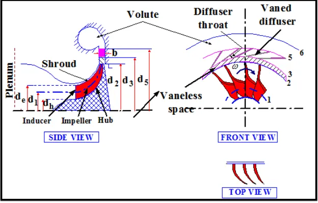
The terminology used to define the components of a

centrifugal compressor is shown in Fig. 1 and the pressure rise across it is depicted in Fig. 2. An enthalpy – entropy diagram is plotted to show the compression process progression in the compressor stage as shown in Fig. 3.

Figure 1. Components of centrifugal compressor.

Figure 2. Pressure rise across the compressor stage.

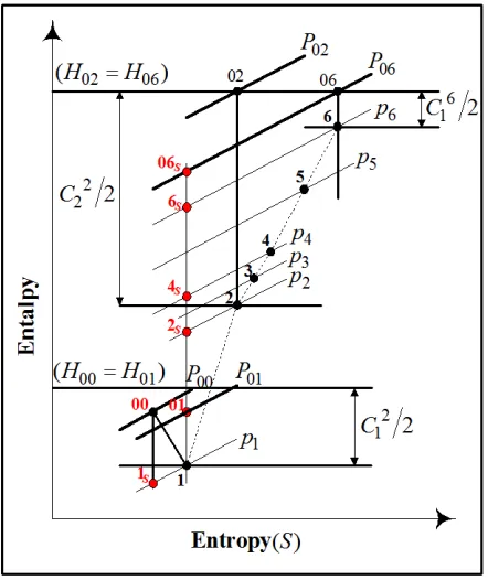
It should be noted that the process departs from isentropic compression due to losses caused by friction, viscous drag and others. In general, the impeller of a centrifugal compressor may be considered as a generalized fluid handling system and

the variables which will completely describe the design and performance of this system may be divided into three groups as shown in Table 1.

Table 1. Main parameters of a centrifugal compressor impeller.

Control variables Design variables Performance requirements

Inlet pressure Tip diameter and blade width Mass flow rate Inlet temperature Inducer and hub diameters Isentropic efficiency Rotational speed Axial length, blade angles Pressure ratio

Figure 3. Generalised H-S diagram for a centrifugal compressor.

For a given set of performance requirements, the design approach entails the calculation of complete geometrical parameters of the impeller, in addition, it is necessary to identify the constraints such as inducer Mach number, temperature and stress limits. The geometric shape of a typical radial flow impeller including the velocity triangles, assuming zero swirl at impeller inlet, are shown in Fig. 4.

Figure 4. A centrifugal impeller with the inlet and outlet velocity triangles.

(i). Impeller Inlet Design Parameters

Before commencing any design procedure, prior knowledge of some parameters must be available, whilst others must be assumed. For an inducer design, prior knowledge is usually

available of; (a) the inlet stagnation pressure and temperature; the standard atmospheric conditions are often applicable, (b) the degree of pre-whirl; here it will be assumed that the flow enters the inducer with zero pre-whirl, (c) the mass flow rate of the working fluid, and (d) it will be assumed that the flow enters uniformly so that there is no variation of axial velocity with radius. In addition using the momentum, continuity and energy equations, several aerodynamic and geometrical expressions of the flow must be derived to evaluate the principal dimensions for the inducer and these are:

a. Speed parameter 2

01

pa

d N C T

 

 

 

 

Considering the flow at the inducer mean diameter, speed parameter is given by:

(

)

1

02 01

2

1 1 1 2

01

1

1 1

( )( )

c s w

pa

P P

d N

c u d d

C T

γ γ π η ϕ

−

 ₋ 

=  

−

 

 

(1)

b. Relative flow Mach number at inducer tip diameter (Mer)

Refer to inlet velocity diagram at inducer tip de in Fig. 4

presented above, the following expressions can be written as:

2 2

2

2 01 2

2 2

2 2

2 01

1

( 1) 1 sin 1

2

e

pa er

e e

pa

d d N

d C T M

d d N

d C T

π

π

γ β

 _{  }

 _{  }

 _{  }

 

=

  _{   } 

 

 _{ } 

− _ −  + _   _

  

 _{ } 

  

 

(2)

Where:

(

)

1

02 01 2

1 2

01

1

1

1

(

)(

)

c s we e

pa

P

P

d N

c

u

d d

C T

γ γ

π η ϕ

−



₋



=





−









(3)

c. Mass flow parameter ₂ 01

2 01

pa

m C T d P

 

 

 

 

ɺ

Using the continuity equation at inducer inlet for mass flow rate gives:

1

01 2 2

2 1

2( 1)

2 2

2 01 ₂

sin ( ) ( )

4

1 ₁

1 ( sin ) 2

pa e h er e

f

er e

m C T d d M

B

d d d P

M

γ γ

β

γ π

γ _γ

β

+ −

 

 

       

= ₋  _{ } _ − __  

 

   _{+ −}  

 

_{ } 

 

ɺ

(4)

d.Inducer tip to impeller tip diameter ratio(de d2)and hub

2

2 2

2 2

01

( 1) cos 1

1 sin

2

e er e

er e pa d M d N d _M C T γ β π γ _β  _{  }  _{ } −   =_{ }  −  ₊   _{  }       (5)

(

)

( )

1

(

)

1 2( 1) 2 01 2 2 01 2 2 2 2 1 1 sin 2 1 sin 4 1 pa er e h e e

f er e

m C T

M d P

d d

d d _d

B M d γ γ γ _β π γ _β γ + − _{ }  −    _{ + }          _  _ =  −_{ }       _   _      _{  } −          ɺ (6) Where:

(

)

(

) (

)

1 1 2 2 2 2 th f e h

n t d B

d d d d

π =

+

 

 

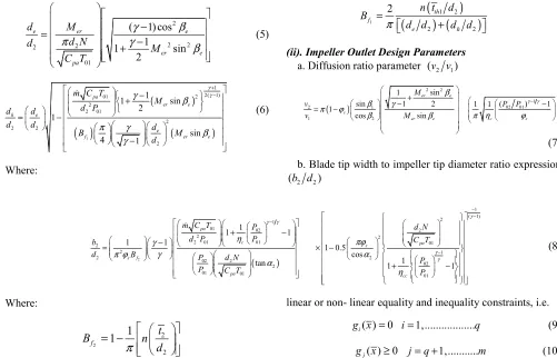
(ii). Impeller Outlet Design Parameters

a. Diffusion ratio parameter (v v_{2 1})

( ) 2 2 1 02 01 2 1 1 2 sin 1

1 2 ( ) 1

sin 1 1

1

cos sin

er e

s

er e c s

M P P v v M γ γ β γ β π ϕ _{β β π η ϕ} −    ₊  _{ }     −  _ − _ = −  _{  }  _  _{  }  _     (7)

b. Blade tip width to impeller tip diameter ratio expression

2 2

(b d )

( )

2

2 1

01 _{02 2}

2 2

01

2 01 01

2 2 1 2 2 02 2 02 2

01 01 ₀₁

1 1 1 1 1 1 0.5 cos 1

tan _{1 1}

pa

c _s pa

s f

pa _cc

m C T P d N

P

d P C T

b

d B _{P d N}

P

P C T _P

γ γ γ γ η _πϕ γ γ α π ϕ α η − −   _{ }      _{+   −}              ₋ _    _     =_ _  _{ } × −   _           _{   }   _{ }  _{+   −}   _{  }  _{ }   ɺ 1 (γ1)

− −                   _   _   _{ }       (8) Where: 2 2 2

1

1

f

t

B

n

d

π









= −





















2.1.2. Optimization Procedure

For a given set of design conditions as listed in Table 2, the optimum geometric dimensions of the impeller were found by solving Eqns. (1) to (8) within the specified ranges of the constraints variables. The solution can be obtained by using a suitable optimisation algorithm. In view of this, numerical optimisation techniques can be a useful tool to problems involving a large number of variables.

Table 2. Compressor input data at design point.

Design Variables Design Values

Mass flow, mɺ_a 0.566

Pressure ratio, P02 P01 4/1

Inlet stagnation temperature, T01 300K

Rotational speed, N 60, 000rpm

Average blade thickness at impeller inlet, t/th2 2.0mm Average blade thickness at impeller outlet, tth1 2.0mm

The authors used the algorithms called optimisation using recursive quadratic programming OPRQP developed by Biggs [29, 30]. The optimisation programme started by assigning different values to a set of parameters X1, X2, X3,...

n

X . Therefore, an objective function denoted by F X( ), where X is a vector with elements, X1, X2, X3,... Xn

must be formulated and the aim is to determine the values of the vector X , which will find the optimum value of the functionF X( ). This function may be subjected to possible

linear or non- linear equality and inequality constraints, i.e.

( ) 0

i

g x = i=1,...q (9)

( ) 0

j

g x ≥ j= +q 1,...m (10)

Where: gi and gj represent non-linear equality and

inequality constraints, respectively. The subscripts i and j

refer to the number of constraints.

(i). Constraint Optimisation Technique Procedure

The frame size and weight of centrifugal compressor is often an important parameter consideration, in view of this, the size of the impeller plays an important rule in determining the overall size of such a compressor. Therefore, the aim is to minimise the impeller tip diameter d2 and this can be

considered a constraint optimisation problem. The procedure to solve such a problem is described below:

a. Selection of main principal parameters of a turbine rotor The choice of selecting the principal parameters of a compressor impeller to solve this optimisation problem is given by the matrix:

2 2 2 2 2 2 1 2 2 1 (1) (2) (3) (4) (5) (6) (7) (8) (9) (10) (11) er e e h d X M X X d d X d d X

X X

b X

b.Formulation of the objective function

The objective function is to optimise the rotor tip diameter and it can be formulated as follows:

Minimize

2

( ) (1)

F X =d =X (12)

c. Formulation of equality and inequality constraints a. Equality constraints

a.1

1

01 2 2

2 1 2( 1) 2 2 2 01 2 sin

(1) ( ) ( )

4

1 ₁

1 ( sin )

2

pa e h er e

f

er e

m C T d d M

g B d d d P M γ γ β γ π γ _γ β + −            = − ₋  _  _{ } − __       ₊ −     _{ }    ɺ (13) a.2 2 1 2 1 ₁

01 _{02 2( 1)}

2 2 2 01 2 01 2

2 02 2 2

01

1 ₁

1 1 ₁

1 1 2 (2) sin pa c f

m C T _P

M P

d P b

g

d B P M

P γ γ _γ γ γ η γ π γ α − ₊ − _{    } _{ } _{  +   − } _{ −  } +          ₋ _     _   = −_  _ _{  }         _{   }       _{  }   ɺ (14) a.3

(

)

2 2 1 02 01 2 1 1 2 sin 1

1 2 ( ) 1

sin 1 1

(3) 1

cos sin

er e

sf

er e c sf

M P P v g v M γ γ β γ β π ϕ β β π η ϕ −    ₊ _{ }    _{ −  − } = − −  _{  } _ _  _{ }  _     (15) a.4 2 2 2 1 1 (4) 234.4 tan sf b N b g d ϕ α −     = −  

   (16)

b. Inequality constraints

b.1 d2≤20.0cm : This is governed by the size of the

compressor

2

(5) 20.0

g = −d (17)

b.2. Mer ≤1.0 : Specified by the subsonic flow requirements

(6) 1.0 er

g = −M (18)

b.3 β ≥_e 25 : Specified by maximum flow at inducer inlet

(7) _e 25

g =β − (19)

b.4 d de 2≥0.55: Governed by the relative Mach number

2

(8) _e 0.55

g =d d − (20)

b.5 dh d2≤0.40 : Specified by stress limitation and

number of blades.

2

(9) 0.40 _h

g = −d d (21)

b.6 α ≥₂ 17 : Controlled by diffusion ratio

2

(10) 17

g =α − (22)

b.7 b2≥0.004: Governed by leakage loss and diffusion

ratio

2

(11) 0.004

g = −b (23)

b.8 v v_{2 1}≥0.55 : Governed by flow separation in the impeller passage

2 1

(12) 0.55

g =v v − (24)

b.9 β ≥2 60 : Specified by diffusion ratio requirements

2

(13) 60

g =β − (25)

b.10 M₂≥0.95: fixed by relative flow angle at impeller exit

2

(14) 0.95

g =M − (26)

b.11 β ≥1 35 : Governed by inducer and hub diameter

1

(15) 35

g =β − (27)

(ii). Optimisation Programme

a general non-linear programming problem using the successive quadratic programming algorithm and a user- supplied gradient. The description of the OPRQP programme is found in Refs. [29-31]. The only unusual feature is the use of the impeller tip diameter d2as an optimisation variable and

an objective function. However, such a choice should not affect the working of the programme.The objective function and the equality and inequality constraints with their first derivatives are inserted into the programme into two sub-routines called, call function and call gradient.

2.1.3. Optimisation Results

The optimisation program was run for a number of blades ranging from 12 to 20. The number of blades was specified within this range in accordance with the assumed efficiency

c

η , blockage B_f and blade loading factor C_w2 u₂ . Fig. 5 shows the impeller tip diameter d₂and the impeller tip width

2

b plotted against the number of blades Nb. As one would

expect, the tip width increases as the diameter is reduced for the blade number from 12 to 15, then the change for both d₂ and b2is fairly small. The design outlet and inlet velocity

diagrams based on optimisation technique are shown in Fig. 6a and 6b. Also, the complete results of the design are given in Table 3a and 3b, respectively.

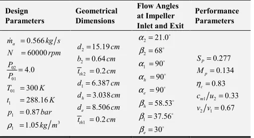
Table 3a. Results data (1) for the impeller based on numerical optimization.

Design Parameters Geometrical Dimensions Flow Angles at Impeller Inlet and Exit

Performance Parameters 02 01 01 1 1 3 1 0.566 60000 4.0 300 288.16 0.87 1.05 = = = = = = = ɺa

m kg s

N rpm P P T K t K p bar kg m ρ 2 2 2 1 1 15.19 0.64 0.2 6.387 3.038 8.506 0.2 = = = = = = = th h e th d cm b cm t cm d cm d cm d cm t cm 2 2 1 1 21.0 68 90 90 90 58.53 37.56 30 = = = = = = = = h e h e α β α α α β β β 1 2 2 1 0.277 0.134 0.83 0.33 0.67 = = = = = P p c m S M c u v v η

Table 3b. Results data (2) for the Impeller based on numerical optimization.

Flow Velocities at Impeller Exit

Flow Velocities at Impeller Inlet

Blade Speed at Impeller Inlet and Outlet Mach Number at Impeller Inlet and Exit 2 2 2 2 2 2 505.35 158.28 412.32 170.71 158.28 63.95 = = = = = = m w m w

c m s

c m s

c m s

v m s

v m s

v m s

1 1 1 1 154.29 0.0 / 154.29 / 154.29 / 253.10 200.65 180.89 308.58 / = = = = = = = = w h e w h e

c m s

c m s

c m s

c m s

v m s

v m s

v m s

v m s

2 1 476.27 / 292.18 / 95.18 / 276.24 / = = = = h e

u m s

u m s

u m s

u m s

2 2 1 1 1.14 0.65 0.453 0.532 0.743 0.903 = = = = = = r hr r er M M M M M M

Figure 5. Plot of impeller tip diameter and tip width against The number of blades.

Figure 6a. Outlet velocity triangle based on numerical optimization technique.

Figure 6b. Inlet velocity triangle based on numerical optimization technique.

2.2. Optimization of Passage Geometry and the Choice of Axial Length

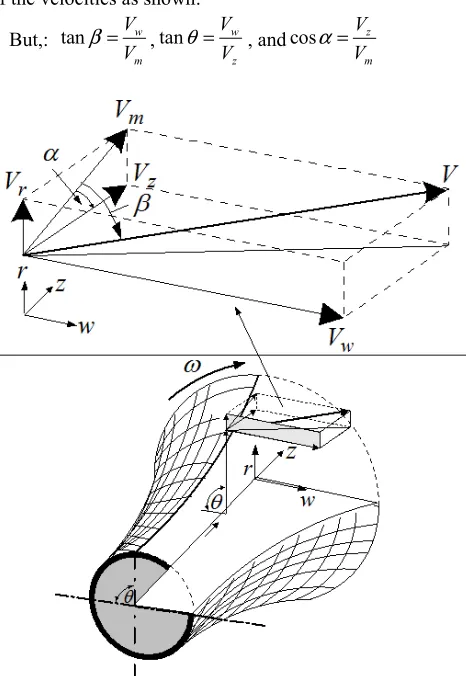
To define the passage geometry of the impeller, the axial length of the impeller is almost a pre-requisite. Therefore, a prescribed mean stream velocity distribution approach was used to optimize the passage geometry and the axial length of the impeller.

impeller passage, as shown in Fig. 7, can be resolved into three basic components along the axial, radial and tangential directions, Vz, Vr and Vw, Here Vm is the velocity vector

along the mean streamline in the hub-to-shroud plane, hence

V = V_z+ Vr+ Vw (28)

The boundary values of the components of the relative velocity are known from the inlet and outlet velocity triangles, which resulted from the previous optimisation. These boundary values are given as follows:

At impeller inlet:

max

( )

z z

V = V

, Vr =0

At impeller exit: 0

z

V = ,Vr =(Vr)max, and Vw= −(1 Cw2 U U2) 2

From Fig. 7, the following relations are hold

z r w

V = + +V V V , V =V_w+V_m (29)

m r z

V = +V V

, Vw=Vsinβ_, Vr =Vmsinα _, Vz =Vmcosα_,

and

1 2 2

sin 1 Vm V

β ₌ − _{− (30)}

The angles shown in Fig. 7 above can be expressed in terms of the velocities as shown:

But,: tan w m

V V

β = ,tan w

z

V V

θ = , andcos z m

V V

α =

Figure 7. Schematic for the relative velocity vector and its components.

The angles (

α

,β and

θ

) are related to each other by combining the above relationships as follows:

tanβ =tan cosθ α (31)

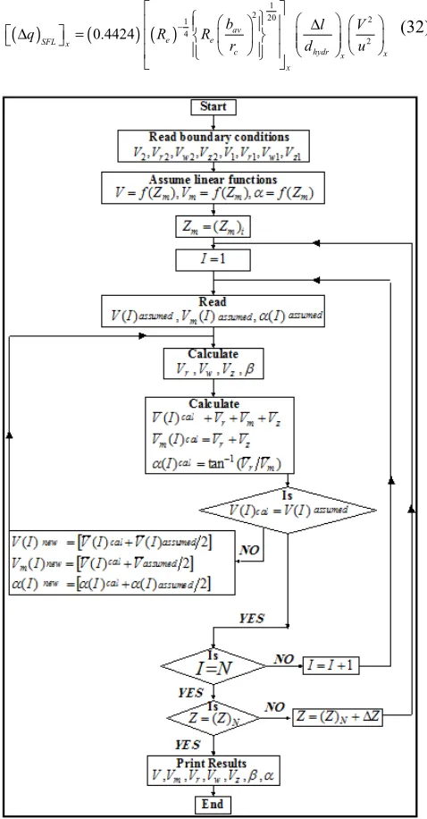
The spatial description of the mean streamline can be found iteratively by assuming a starting value for the meridional length z_m, and the distributions of the relative velocity vector.

Figure 8 describes the velocity componentsVr, Vz and Vw

for one assumed value of Z=0.06m. At the start, all these figures are based on the assumption that the variation of the relative velocity vector V is linear. A computer program was written to perform the iterative calculations to check this linear relationship variation of relative velocity vectors along the mean streamline and the flow angles

α

andβ . The output results are plotted in Fig. 9 and 10, and a flow chart based on this program is shown in Fig. 11.

Figure 8. Assumed linear relationship of relative velocity vector mean and its components for an assumed Z=0.06m_.

Figure 9. Prescribed relative velocity distribution along streamline for an assumed meridional length of zm=0.06m .

2.3. Loss Models

Several models are available in the published literature Dallenbach [32] and Rodgers [33] which takes account of the losses. These loss models were adopted for the impeller as given in Eqns. 32 and 33, respectively. A detailed review and derivation of these loss models are outside the scope of this paper, but it should be mentioned that any loss models might be integrated into the program as sub-routine.

2.3.1. Skin Friction Loss

Skin friction loss expression at any section

X

as a dimensionless quantity is given by:

( )

(

) ( )

1

2 20 2

1 4 2 0.4424 av e e SFL x

c hydr x x

x

b l V

q R R

r d u

−               _∆ _∆  ₌             _{   }  _{  }         (32)

Figure 11. Flow chart for relative velocity vector variation along mean streamline.

2.3.2. Combined Diffusion and Blade Loading Losses

Combined diffusion and blade loading losses expression at any section

X

as a dimensionless quantity is given as:

( )

2

1 1

sin

0.05 1 1

2 2

x

DBL x

x x

v d du

q

v l lv

π β π         ∆  =  −  +  +     _{ ∆  ∆}         (33)

2.3.3. Shock Losses

These losses are ignored as the flow is subsonic. The next step was to optimize the axial length

Z

by minimizing the loss of stagnation pressure in the flow channels. Therefore, a computer program was written to optimize the axial length and the flow passage based on the relations listed here. Here the radius r of the mean streamline in the meridional plane can be represented using Lame’ ovals relationship as:

(

)

1 3 2 1 2 2 2 1

1 m m

m m

z z

r r r r

z z  _{ − }    = − −  + −       (34)

The first and second derivatives of dr dz are given in Eqns. 35 and 36, respectively:

2 1

1

1 2 2

2 1 2 1 1 2

3 2

m m

m m m m

z z

r r r r

dr l

dz z z j z z r r

−

 ₋   ₋   ₋ 

 

= −_{ }     

− − −

       (35)

2

2

1 2

2 1

m m m m

m

d r dr dr

dz z z r r dz dz        ₋   =  +   − −    

      (36)

The length of the streamline is given by:

2 1 1 2 1 m m z m m z dr L dz dz   =  +   

∫

(37)

The temperature at any section

X

inside the passage

2 01 01 1 2 x x pa u T T C T   = _ + _

  (38)

The pressure at any section

X

inside the passage

1 01 01 x x s P T P T γ γ ϕ −   = 

  (39)

The density at any section inside the passage

1 1 2 1 2 x x x

p x x

v P

C T RT

γ

ρ = −_ _ −  

 

 

(40)

The shroud contours at any section

X

inside the passage

2 1 cos

( )

2

a x

sx rms x

x mx fx

m

r r

v B

α π ρ

= + ɺ (41)

The hub contours at any section

X

inside the passage

2 2

(2 )

hx rms x sx

It can be seen from Eqns. 27 and 28 that they can be used to calculate the shroud and the hub contours at any section

X

inside the blade passage, hence the final shape of the blade passage can be defined. A flow diagram for optimising the axial length and flow passage of the impeller is given in Fig. 12. The output results are presented graphically. Fig. 13 shows a plot of impeller internal losses, that is, skin friction losses

SFL

q

∆ and diffusion and blading losses ∆qDBL vs. meridional

length of a centrifugal impeller. As one would expect that

SFL

q

∆ is lowest for the smallest axial length and increases as the axial length is increased while ∆qDBL is highest for the

smallest axial length and decreases as the axial length is increased. Figure 14 shows a plot of total pressure loss inside the passage vs. meridional length of a centrifugal impeller. It can be seen that the optimum meridional length was found to be 41.5mm for minimum pressure loss in the passage.

Figure12. Flow chart for the design of the flow passage and optimizatio of the meridional length.

Figure 13. Variations of impeller internal losses along theimpeller passage.

Figure 14. Overall impeller internal losses along the impeller passage.

Figure 15. Three dimensional solid model of the designed impeller.

2.4. Validation of the Optimization Code

The aim of this validation is to check the reliability of present code to be used with confidence for the flow analysis. The data published by Eckardt [34] and Tough et al. [35] were chosen to validate the present code. Eckardt [34] performed measurements for detailed investigation of flow field in a centrifugal impeller. The measured data have been widely used to validate computational codes and also quoted

in describing the flow characteristics along the impeller. Tough et al. [35] carried out a CFD analysis to determine the solution of the flow of a centrifugal impeller. Results of present calculations of the geometric parameters in this work show quite good agreement with the published work in the open literature [34, 35]. The discrepancies between the results can be attributed to the different input parameters of the impellers as shown in Table 5.

Table 4. Geometric parameters of Eckardt impeller and Tough et al. [35].

Parameter Proposed impeller Tough et al. [35] Impeller (CFD analysis) Eckardt [34] impeller (computational code) Inlet tip diameter dt=8.506cm dt=5.48cm dt=28cm

Inlet hub diameter dh=3.038cm dh=2.87cm dh=9.0cm

Outlet diameter d2=15.9cm d2=9.52cm d2=20cm

Impeller exit width b2=0.64cm b2=0.32cm b2=2.6cm

Inlet blade angle β1=37.6 β1=30.0 β1=30.0

Pressure ratio Pr=4.0 Pr=4.2 Pr=4.3

Mass flow rate mɺ=0.566kg s mɺ=1.45kg s mɺ=5.31kg s

Inlet total temperature 300K 288K 288K

Table 5. Comparison of results between the proposed impeller with Eckardt [34] and Tough et al. [35] impellers.

Parameter Proposed impeller Tough et al. [35] impeller Eckardt impeller [34]

Numerical results CFD results Measured results

Inlet absolute velocity c1=154.29m s c1=136.30m s c1=135.90m s

outlet absolute velocity c2=505.35m s c2=403.90m s c2=470.74

Inlet relative velocity v1=253.10m s v1=268.50m s v1=263..20m s

Outlet relative velocity v2=170.71m s v2=175.40m s v2=180.25m s Inlet relative Mach number Mr1=0.743 Mr1=0.797 Mr1=0.78

Outlet relative Mach number Mr2=0.65 Mr2=0.61 Mr2=0.60

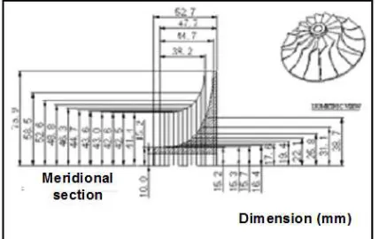
Figure 17. Detail design drawing of the designed impeller.

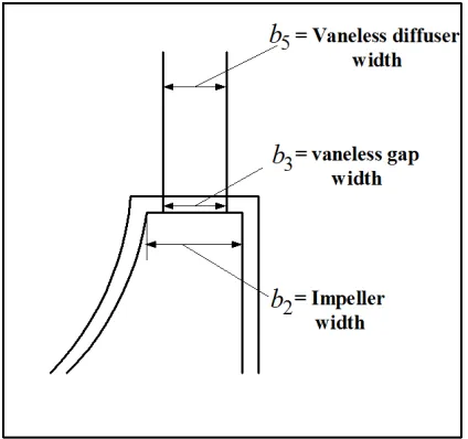
3. Vaneless Diffuser

The vaneless diffuser is often adopted as the sole means of pressure recovery owing to its simplicity and inexpensive construction, its broad operating range and its ability to reduce

is unsatisfactory. The vaneless diffuser may be a vaneless space between the impeller tip and the beginning of a channel or cascade diffuser or it may be run from the impeller discharge to the volute inlet. Analysis in the previous section showed that the fluid discharges from the impeller at high velocity, see Table 3, and consequently it is essential to convert the kinetic energy efficiently into static pressure. The vaneless diffuser considered in the current paper is two parallel walls forming an open passage from the impeller tip to a specified discharge diameter as shown in Fig. 18. The following section describes the design procedure.

Figure 18. Reduced width in vaneless gap of a centrifugal compressor casing.

Vaneless Diffuser Design Analysis

The flow at entry to the vaneless diffuser is extremely complex, consisting of jet and wakes issuing from each passage of the impeller Dean and Senoo [19]. Therefore, mixing out occurs as the flow leaves the impeller tip at a finite radial increment outside impeller known as the vaneless gap where the flow is exposed to sudden enlargement forming eddies and friction losses. Fisher [36] gives a diameter ratio of the vaneless gap to the impeller tip d₃ d₂ is equal to 1.1 to reduce non-uniformity and noise. The simplest description of the flow through the vaneless diffuser can be obtained by considering the angular momentum equation used for the impeller but applied between the impeller exit (2) and the vaneless diffuser exit (5), (refer to Fig. 2), that is

5 5 2 2

( )

m c r_ω c r_ω

τ = ɺ − (43)

For the case of an open passage where the flow is only retained by the side walls and in the absence of any wall friction force, the torque

τ

exerted on the fluid is zero and the angular momentum equation above reduces to free vortex relationship

5 5 2 2

c r_ω =c r_ω (44)

At any station along the diffuser in relation to impeller exit, the above equation is written as:

2 2

c r_ω =c r_ω or c dω =c dω2 2 (45)

Applying mass continuity at any station along the diffuser in relation to impeller exit would give:

2 2 m2 m

mɺ =ρ A c =ρAc

2 2 2tan 2 tan

mɺ =ρ A c_ω α =ρAc_ω α (46)

Combining equations 45 and 46 with the equation of state

p=ρRT and substituting for A2 b d2 2

A db

π π

= and re-arranging

would give an expression for static pressure ratio in the vaneless diffuser: 2 2 2 2 tan tan b p t

p t b

α α

    

=    

   

  (47)

For adiabatic condition in the vaneless diffuser, temperature ratio in the vaneless diffuser can be expressed as:

2 02 2 2 2 02 1 2 1 2 pa pa c C T t t c C T − = − (48)

and from general velocity triangle, the velocities cand c₂ can be expressed as

2(2 )

cos cos

c c r r

c ω ω

α α

= = and 2

2 2 cos c c ω α

= (49)

Substituting for c₂ and c expressions in Eqn. 49 and combining with Eqns. 47 and 48 will give an expression for static pressure rise ratio within the vaneless diffuser as:

2 2

2 2

02 2 2

2 2 ₂ 2 02 cos 1 2 tan tan cos 1 2 pa pa c r r

C T b

p

p _c b

C T ω ω α α α α  _{   }   _{   }   ₋             =_{    }   _    _{ }   ₋       (50)

For parallel wall vaneless diffuser, the width b= =b₃ b₅, hence Eqn. 50 becomes:

2 2

2 2

02 2 2

2

2 ₂ 5

2 02 cos 1 2 tan tan cos 1 2 pa pa c r r

C T b

p

p _c b

C T ω ω α α α α  _{   }   _{   }   ₋      _{   }    =_{ }  _ _      _{ }   ₋       (51)

vaneless diffuser is a function of radius ratio r r2 and the

absolute flow angle

α

. For an efficient diffusion, the flow angle

α

must be reduced with increasing radius ratio. Eqn. 51 is plotted as shown in Fig. 19 to show the variation of pressure recovery in the vaneless diffuser. Figure 20 shows the variation of both the tangential and radial velocities with radius ratio in the vaneless diffuser. It can be seen that both velocities are decreasing with increasing radius ratio. The final design data of the vaneless diffuser parameters at exit are given in Table 6.

Figure 19. Pressure rise in the vaneless diffuser.

Figure 20. Variation of tangential and radial velocities with radius in the vaneless diffuser.

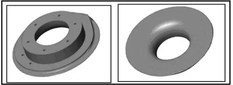
The final design drawing of the vaneless diffuser is shown in Fig. 21 and a three-dimensional solid model of the vaneless diffuser is shown in Fig. 22.

Figure 21. Detail design drawing of the vaneless diffuser.

Figure 22. Three dimensional solid model of the vaneless diffuser.

Table 6. Complete design data of vaneless diffuser.

Design parameters Design values

Vaneless diffuser diameter, d5 22.026cm Vaneless diffuser width, b5 0.582cm Static pressure at exit, p5 3.88bar Flow angle at exit, α5 12.55 Tangential velocity at exit, cω5 284.36m s Radial flow velocity at exit, cr5 63.37m s Absolute flow velocity at exit, c5 291.33m s Static temperature at exit, t5 430.28 K

Density at exit, ρ5

3

3.14kg m

4. Volute Design

The last basic component of a centrifugal compressor stage is the volute or scroll. It is a spiral – shaped housing which collects the flow from the diffuser and passes it to a pipe at the exit.

Design Method

Considering the flow in the volute to be frictionless and the volute cross-section to be circular, for simplicity and ease of manufacture, the continuity equation at azimuth angle φ gives:

mɺ_φ =ρ_{φ φ ωφ}A c (52)

But

360

m_φ =m φ 

 

ɺ ɺ

Since the difference in velocity at r₅and r_φ is likely to be small compared to the local velocity of sound, then the density ratio will be nearly one, consequently;

4 φ

ρ =ρ , c_ωφ =c_ω and

2

4

d A_φ =π φ

Substituting the above expressions in Eqn. 52 and re-arranging will give an expression for volute cross-section diameter at any azimuth angle as:

1 2

4 360

m d

c

φ

φ ωφ

φ

π

ρ

_{  } 

=_{  } _

  

  

 

ɺ

(53)

Figure 23. Detail design drawing of the volute.

Figure 24. Detail design drawing of the volute cover.

A three dimensional solid model of the volute and its cover are shown in Fig. 25 and Fig. 26., respectively.

Figure 25. Multiple views of three- dimensional solid modelthe volute cover.

Figure 26. Multiple views of three- dimensional solid model of the volute.

FINAL DESIGN MODEL OF THE COMPRESSOR Final design drawing and three-dimensional solid model and an exploded view representation of the centrifugal compressor assembly are shown in Figs. 27, 28 and 29, respectively.

Figure 27. Schematic diagram of the centrifugal compressor assembly.

Figure 28. Exploded view of the centrifugal assembly.

5. Conclusion

a)The design of a single stage centrifugal compressor comprising an impeller, a vaneless diffuser and the volute has been presented. The compressor has been designed as part of micro-gas turbine designed for power generation running at 60000rpm and developing

60kW electrical power.

b)The principal geometric dimensions of the impeller and the number of blades were determined based on non-linear optimization code developed for this purpose. Also, the code was used to find the optimum axial length and optimizing the blade passage.

c)The computer code for the design of the impeller was verified and the results showed quite good agreement with CFD analysis published data in the open literature. d)A procedure for designing the vaneless diffuser and the

volute was given based on the governing equations of mass, momentum, and energy conservation. The flow is assumed to be isentropic and satisfies the free vortex relationship.

Notation

A

Area normal to mean flow direction ( 2

m )

b Blade width (m)

f

B Blockage factor

C Absolute flow velocity of gas (m s)

p

C Specific heat capacity at constant pressure for gas

(kJ kgK)

d Diameter (m)

c

f Friction factor

M

Absolute Mach number

r

M Relative Mach number mɺ Mass flow rate (kg s) N Rotational speed (rpm)

b

N Number of blades

P

Stagnation pressure (N m2, bar)

e

R Reynolds number

c

r Radius of curvature ( )m

T

Stagnation temperature (

K

)

t

Blade thickness ( )m

u Impeller tip velocity (m s) ,

v V Relative velocity (m s) W Work output (kJ)

z Axial length ( )m

Greek Symbols

α

Absolute flow angle relative to axial direction (degree), angle between meridional streamline and axis

β Relative flow angle relative to axial direction

(degree), angle between relative velocity vector and meridional plane

b

β Blade angle

θ

Relative angular co-ordinate

γ

Ratio of specific heats

η

Efficiency of a process

ρ

Gas density (kg m3)

ψ

Blade loading

ϕ

Pressure loss coefficient

s

ϕ Slip factor

φ Centroid

ω

Angular velocity (rad s)

∆

Small increment of

Subscripts

0 Stagnation conditions 1 Impeller inlet station at mean 2 Impeller outlet station 3 Vaneless diffuser inlet station 5 Vaneless diffuser outlet station

a Air

av Average

c Compressor

e Exit condition

h Hub

hydr Hydraulic diameter i Inlet condition

m Mean

SFL Skin friction loss

DBL

Blade loading coefficient w Tangential direction rms Root mean square

r Radial direction

x Any station inside the rotor passage

References

[1] Japikse, D. “Decisive factors in advanced centrifugal compressor design and development,” in Proceedings of the International Mechanical Engineering Congress & Exposition, Nov. 2000.

[2] Xu C., Amano R. S., “Development of a low flow coefficient single stage centrifugal compressor,” International Journal of International Journal of Computational Methods in Engineering Science and Mechanics, Vol. 10, 2009, pp. 282– 289.

[3] Aungier R. H., “Centrifugal Compressors—A Strategy for Aerodynamic Design and Analysis”. ASME Press, New York, NY, USA, 2002.

[4] Xu C., “Design experience and considerations for centrifugal compressor development,” Proceedings of the Institution of Mechanical Engineers, Part G, Vol. 221, 2007, pp. 273–287. [5] Cosentino R., Alsalihi Z., Braembussche V. R. A., “Expert

[6] Perdichizzi A., Savini M., “Aerodynamic and geometric optimization for the design of centrifugal compressors”. International Journal of Heat and Fluid Flow, Vol. 6, issue 1, March 1985, pp. 49–56.

[7] Al-Zibaidy S. N., “A proposed design package for centrifugal impellers”. Computers and structures, Vol. 55, issue 2, April 1995, pp. 347–356.

[8] Xu C., Amano R. S., “Empirical Design Considerations for Industrial Centrifugal Compressors”. International Journal of Rotating Machinery, Vol. 2012, 15 pages.

[9] Cho S. Y., Ahn K. Y., Lee Y. D., Kim Y. C., “Optimal Design of a Centrifugal Compressor Impeller Using Evolutionary Algorithms”. Mathematical Problems in Engineering, Vol. 2012, 22 pages.

[10] Ibaraki S., Sugimoto K., Tomito I., “Aerodynamic design optimization of a centrifugal compressor impeller based on an artificial neural network and genetic algorithm” Mitsubishi Heavy Industries Technical Review, Vol. 52, 1, March, 2015. [11] Bonaiuti D., Arnone A., Ermini M., Baldassarre L., “Analysis

and optimization of transonic centrifugal compressor impellers using the design of experimental technique,” GT-2002-30619, 2002.

[12] Verstraete T., Alkaloid Z., Van den R. A., “Multidisciplinary optimization of a radial compressor for microgas turbine applications,” Journal of Turbomachinery, Vol. 132, 3, 2010, 7 pages.

[13] Ingham, D. R. and Bhinder, F. S., “The effect of inducer shape on the performance of high pressure ratio centrifugal compressors”. ASME paper, No. 74-GT-122, 1974.

[14] Stahler, A. F., “Transonic flow problems in centrifugal compressors”. SAE, preprint No. 268C, Jan. 1961.

[15] Polikovsky, V. and Nevelson, M., “The performance of a vaneless diffuser fan”. NACA. TM 1038, 1942.

[16] Brown, W. B. “Friction coefficient in a vaneless diffuser”. NACA. TN 1311, 1947.

[17] Brown, W. B. and Bradshaw, G. R. “Methods of designing vaneless diffusers and experimental investigation of certain undetermined parameters”. NACA. TN 1426, 1947.

[18] Stantiz, J. D. “Some theoretical aerodynamic investigations of impellers in radial and mixed flow centrifugal compressors”. Transaction of ASME 74:374, 1952.

[19] Dean, R. C., Senoo, Y. “Rotating wakes in a radial vaneless diffuser”. ASME., Series D, Sept. 1960.

[20] Johnston, J. R., Dean, R. C. “Losses in vaneless diffuser on centrifugal compressors and pumps” Transaction ASME, Journal of engineering for power, Vol. 88, No. 1, Jan. 1966. [21] Bettini C., Cravero C., Rosatelli F., Zito D., "The Design of the

centrifugal Compressor for a 100kW micro gas turbine power plant".

[22] Zahed A. H., Bayomi N. N., “ISESCO Journal of Science and Technology”, Vol. 10, 17, 2014, pp. 77-91.

[23] Marefat A., Shahhosseini M. R., Ashjari M. A. "Adapted design of multistage centrifugal compressor and comparison with available data", International Journal of Materials, Mechanics and Manufacturing. Vol. 1, 2, May 2013. [24] Kurauchi S. K. Barbosa J. R. "Design of centrifugal

compressor for natural gas". Vol. 12, 2, 2013, pp.40 -45. [25] Li P. y., Gu C. W., Song Y. "A new optimization method for

centrifugal compressors based on 1D calculations and analysis". Energies. Vol. 8, 2015, pp. 4317-4334.

[26] Gui F., Reinarts T. R., Scaringe R. P., Gottschlich J. M., "Design and experimental study on high speed low flow rate centrifugal compressors". IECECP, paper No. CT-39. [27] Moroz L., Govoruschenko Y., Pagur P., Romaneko L.

"Integrated conceptual design environment for centrifugal compressors flow path design". Proceedings of IMECE, 2008. [28] Bowade A., Parashhkar C. "A review of different design

methods for radial flow centrifugal pumps". International Journal of Scientific Engineering and Research (IJSER). Vol. 3, 7, 2015.

[29] Biggs, M. C., “Recursive quadratic programming methods for non-linear constraints”. In Powel, M. J. C., ed., “Nonlinear optimization”. 1981.

[30] Biggs, M. C., “Further methods for nonlinear optimization”. Mathematics division, University of Hertfordshire, 1999. [31] Numerical optimization centre. “Optima manual”. School of

Information sciences, Hatfield Polytechnic. Issue No.8, July 1989.

[32] Dallenbach, Coppage et al. “Study of supersonic radial compressors for refrigeration and pressurization”. WADC Techincal Report 55-257, A. S. T. I. A document No. AD110467, Dec 1956.

[33] Rodgers C., A diffusion factor correlation for centrifugal impeller stalling, Trans. ASME. Jr. of Eng. for Power, Vol. 100. Oct, 1978.

[34] Eckardt D. “Detailed flow investigations within a high-speed centrifugal compressor impeller”, Trans. ASME, September, 1976.

[35] Tough R. A., Tousi A. M., Ghaffari J., “Improving of the micro-turbine's centrifugal impeller performance by changing the blade angles”. ICCES, Vol. 14(1), pp. 1-22, 2010. [36] Fisher, F. B., “Development of vaned diffuser components for