Proc. IAHS, 379, 335–341, 2018
https://doi.org/10.5194/piahs-379-335-2018 © Author(s) 2018. This work is distributed under the Creative Commons Attribution 4.0 License.
Open Access
Inno
v
ativ
e
w
ater
resources
management
–
understanding
and
balancing
inter
actions
betw
een
humankind
and
n
ature
Multi-model ensemble hydrological simulation
using a BP Neural Network for the
upper Yalongjiang River Basin, China
Zhanjie Li1,2, Jingshan Yu1,2, Xinyi Xu1, Wenchao Sun1,2, Bo Pang1,2, and Jiajia Yue3
1College of Water Sciences, Beijing Normal University, Beijing 100875, China
2Beijing Key Laboratory of Urban Hydrological Cycle and Sponge City Technology, Beijing 100875, China
3School of Geographical Science, Qinghai Normal University, Xining 810016, China
Correspondence:Jingshan Yu ([email protected])
Received: 20 November 2017 – Revised: 31 March 2018 – Accepted: 3 April 2018 – Published: 5 June 2018
Abstract. Hydrological models are important and effective tools for detecting complex hydrological processes. Different models have different strengths when capturing the various aspects of hydrological processes. Rely-ing on a sRely-ingle model usually leads to simulation uncertainties. Ensemble approaches, based on multi-model hydrological simulations, can improve application performance over single models. In this study, the upper Ya-longjiang River Basin was selected for a case study. Three commonly used hydrological models (SWAT, VIC, and BTOPMC) were selected and used for independent simulations with the same input and initial values. Then, the BP neural network method was employed to combine the results from the three models. The results show that the accuracy of BP ensemble simulation is better than that of the single models.
1 Introduction
Hydrological processes are complex and are affected by many factors, including climate, weather, topography, and the sub-surface. Hydrological models provide important and effective methods of hydrological research for describing complex water cycle processes. Because of the different structure of each model, their simulation ability for a hydro-logical process is also different. Each hydrohydro-logical model has its own characteristics and basins where it can be more effec-tively applied. Relying on a single model often leads to pre-dictions that capture some phenomena at the expense of oth-ers (Duan et al., 2007). Multi-model ensemble hydrological simulation has been an effective method for improving simu-lation accuracy. Many researchers have applied multi-model simulation methods to improve the simulation and prediction accuracy of hydrological models (Ajami et al., 2007; Devi-neni et al., 2008; Najafi and Moradkhani, 2016; Razavi and Coulibaly, 2016; Zhu et al., 2016).
Artificial neural networks (ANNs), as an abstraction and simulation of some of the basic characteristics of human brain or natural neural networks, have received great
atten-tion because of their advantages in solving highly nonlinear problems of great social concern. The “feed-forward, back propagation” neural network (BPNN), which is currently the most popular network architecture, can be applied in a vari-ety of fields according to the characteristics of the model (Hu et al., 2005; Yaseen et al., 2015). Wei et al. (2013) established a predictive model, based on a wavelet-neural network hybrid modelling approach, for monthly river flow estimation and prediction (Wei et al., 2013). Wang et al. (2017) proposed a new back-propagation neural network algorithm and applied it in the semi-distributed Xinanjiang (XAJ) model. The im-proved hydrological model was capable of updating the flow forecasting error without losing the lead time (Wang et al., 2017).
Table 1.Weather stations in the basin.
Station name Latitude (N) Longitude (E) Elevation (m)
Qingshuihe 97◦080 33◦480 4415.4
Shiqu 98◦060 32◦590 4200.0
Shiquluoxu 98◦000 32◦280 3242.1
Ganzi 100◦000 31◦370 3393.5
Seda 100◦200 32◦170 3893.9
Daofu 101◦070 30◦590 2957.2
Xinlong 100◦190 30◦560 3000.0
Litang 100◦160 30◦000 3948.9
Qianning 101◦290 30◦290 3449.0
predictions using the BP schemes. Section 5 provides sum-maries and conclusions.
2 Study area and data collection
2.1 Study area
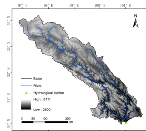
The Yalongjiang River (YLJR) is located in the Sichuan Province in southwestern China, in the eastern Tibetan Plateau, and is the largest tributary of the Jinshajiang River in the upper Yangtze River. The total length of the main stream of YLJR is 1571 km, and the YLJR Basin area is about 128 440 km2, accounting for 13 % of the total area of the upper reaches of the Yangtze River. The average annual runoff in the YLJR Basin is about 58 billion m3. The upper reaches of the YLJR Basin, above the Yajiang in situ gauging station, were selected as the study area.
The terrain elevation of the upper YLJR Basin varies greatly and from north to south ranges from 2600 to 6111 m. Because of the influence of the westerly atmospheric circu-lation and monsoons, the north-south climate change is also very obvious, with a dry continental climate in the northern plateau and a subtropical climate in the central and south-ern parts of the basin. The winters are long and cold, and the summers are cool and wet, with strong radiation all year round. The average annual precipitation during the last 50 years was about 500–2470 mm, of which 73 % occurred from June to September. The inter-annual change, and re-gional distribution trend, of streamflow in this basin is similar to the precipitation.
2.2 Data description
The Digital Elevation Model (DEM) dataset was taken from the Computer Network Information Centre, Chinese Academy of Sciences (http://www.gscloud.cn, last access: 17 April 2018), was used to derive the mean elevation and slope of the region at a resolution of 90 m. The land cover datasets in this study were determined using MODIS (MOD12Q1-051) data (https://lpdaac.usgs.gov, last access: 17 April 2018), and included grassland, woodland, cropland, urban and built-up areas, water, and unused land. In 2010,
Figure 1.Topography, river networks, and streamflow gauging sta-tion of the basin.
approximately 89 % of the entire study area was covered by grassland; woodland covered approximately 9 %, and the re-mainder was covered by other land cover types. The soil map for the basin was derived from the Chinese national 1:1 000 000-scale soil map. The physical properties of these soils were obtained from the China Soil Scientific Database (http://www.soil.csdb.cn/, last access: 17 April 2018). The other properties used as parameters for the models were com-puted using empirical equations (Saxton, 2006). The main soil type is plateau meadow soil.
There are nine national weather stations in the basin, shown in Table 1. Daily meteorological records from these stations for 1960 to 2013 were used to assess the perfor-mance of a range of probability distribution models (http: //data.cma.cn/, last access: 17 April 2018). Daily Streamflow data for the basin (Yajiang station) for 2007 to 2011 were ob-tained from the Institute of Geographic Sciences and Natural Resources Research, Chinese Academy of Sciences (CAS). These data were used to calibrate the model parameters. The topography, river networks, and streamflow gauging station of the basin are presented in Fig. 1.
3 Methodology
3.1 Hydrological models
For this study, we employed three kinds of common dis-tributed hydrological models (SWAT, VIC, and BTOPMC) as the ensemble members of multi-model simulation.
Table 2.SWAT model parameters calibrated.
Name Description Initial range
CN2 SCS runoff curve number 20–90
SLSUBBSN Average slope length (m) 10–150
ALPHA_BF Baseflow recession coefficient 0–1
GW_DELAY Groundwater delay time (days) 30–450
EPCO Plant uptake compensation factor 0.01–1
OV_N Manning coefficient for overland flow 0–0.8
ESCO Soil evaporation compensation coefficient 0.8–1
CH_K2 Hydraulic conductivity in main channel (mm h−1) 5–130
SOL_AWC Available soil water capacity (mm H2O mm Soil−1) 0–1
SOL_K Soil saturated hydraulic conductivity (mm h−1) 0–2000
SNOCOVMX Threshold depth of snow, above which there is 100 % cover 0–500
SNO50COV Fraction of snow volume represented by SNOCOVMX that corresponds to 50 % snow cover 0–1
Table 3.Parameter values for the VIC model.
Name Description Initial range
B Exponent of variable
infil-tration capacity curve
0–10.0
D Fraction of maximum base
flow
0–1.0
Dmax Maximum velocity of base
flow (mm day−1)
0–30
Ws Fraction of maximum soil
moisture content of the third layer
0–1.0
d1,d2,d3 three soil layer thicknesses
(m)
0.05–2.0
and transportation of sediment and pollutants at the basin scale. The hydrological processes considered in the model include precipitation, interception, infiltration, evapotranspi-ration, snowmelt, surface runoff, percolation, baseflow, and flow movement in river channels. The model divides a basin into multiple sub-basins that are further subdivided into hydrological response units (HRUs), which have homoge-neous land use and soil characteristics. Three steps are in-volved in simulating the hydrological processes: (1) prepar-ing the meteorological input and GIS data of the soil type and land cover, (2) constructing the model, and (3) the cali-bration/validation process. In the present study, 12 sensitive parameters were identified for model calibration using the GLUE (Beven and Binley, 1992) method. The parameters are described and listed in Table 2.
VIC (Variable Infiltration Capacity) (Liang et al., 1994) is a large-scale, semi-distributed land surface hydrological model that solves full water and energy balances, and was originally developed at the University of Washington. It is a grid-based, soil-vegetation-atmosphere transfer scheme that clearly reflects the effects of infiltration, precipitation, and the spatial variability of vegetation on water fluxes through
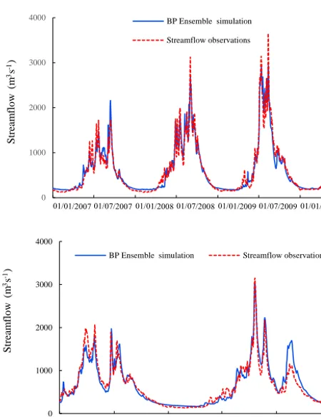
Table 4.Parameters of BTOPMC model.
Name Description Range
m Decay factor 0.005–0.1
α Drying function parameters −10–10
Sbar0 Average soil saturation deficit (m) 0.001–0.9
D0 Coefficients of discharge ability 0.1–200
Srmax Maximum storage capacity of root zone (m) 0.001–0.8
n0 Block average Manning’s coefficient −2.0–2.0
the landscape. The model takes into account the spatial, sub-grid scale, variability of infiltration, precipitation, and veg-etation. The newest version of the VIC model consists of three layers that allow for explicitly depicting the dynam-ics of surface and groundwater interactions, and calculat-ing the groundwater table (Liang et al., 2003). The model is driven by data on precipitation, maximum and minimum daily temperature (daily-time step), vegetation type, and soil texture. The generated runoff is routed laterally using simu-lated topology and stream networks to the basin outlet. The parameters and their initial prior ranges are briefly described in Table 3.
Figure 2.The topology of the BPNN model.
Table 5.Comparison between ensemble simulation and ensemble
members’ optimal simulating series.
SWAT VIC BTOPMC BP Ensemble
ENS Calibration 0.77 0.75 0.82 0.95
Validation 0.66 0.65 0.75 0.90
3.2 BP neural network
The BPNN is a multilayer structure and feed forward map-ping model trained by an error back propagation algorithm. The topology of the BPNN model mainly comprises the in-put, hidden, and output layers. The BP algorithm consists of forward propagation and error back propagation. In the for-ward propagation, the input information is processed from the input layer to the output layer through the hidden layer. The state of each layer is only affected by the state of the next layer. If the expected output is not obtained in the output layer, then it is transferred back to the error back propagation. The error signal is returned along the original connection path. The error is minimized by modifying the weights of each layer node. The topology of the BPNN model is shown in Fig. 2.
In the present study, the inputs of the BP network are the simulation results of three hydrological models, and the out-put is the streamflow at the Yajiang station.
3.3 Model performance indicators
Before the model can be applied for evaluating the method proposed in this study, the model robustness in the basin must be examined by assessing the model’s performance in terms of benchmark calibrations. The Nash–Sutcliffe efficiency co-efficient was selected to evaluate the simulation performance of the three individual models as well as multi-model ensem-ble simulation:
ENS=1−
n
P
i=1
Qobs,i−Qsim,i2
n
P
i=1
Qobs,i−Qobs,avg2
, (1)
0 1000 2000 3000 4000
S
tr
ea
m
fl
o
w
(
m
s
)
3
-1
SWAT simulation
Streamflow observations
0 1000 2000 3000 4000
S
tr
ea
m
fl
o
w
(
m
s
)
3
-1
SWAT simulation
Streamflow observations
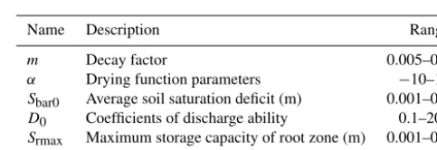
Figure 3.SWAT simulated streamflow for the basin in both the
calibration and validation periods.
whereQobs,i (m3s−1) andQsim,i (m3s−1) represent the
ob-served and simulated streamflow, respectively, at time stepi, andQobs,avg(m3s−1) is the average value of the streamflow observations. The integern is the number of samples.ENS measures the agreement between modeled and observed val-ues, withENS=1.0 indicating a perfect agreement between modeled and observed streamflow for a given basin.
4 Results and discussion
4.1 Streamflow simulation of each ensemble member
Using available streamflow records, the benchmark calibra-tion for the basin was conducted using continuous daily streamflow observations for 1 January 2007–30 April 2010, and was validated using data for 1 May 2010–31 Decem-ber 2011. The results of the benchmark calibrations of the three ensemble members are listed in Table 5, and the stream-flow simulations are shown in Figs. 3–5.
0 1000 2000 3000
4000 VIC simulation
Streamflow observations
0 1000 2000 3000
4000 VIC simulation
Streamflow observations
S
tr
ea
m
fl
o
w
(
m
s
)
3
-1
S
tr
ea
m
fl
o
w
(
m
s
)
3
-1
Figure 4.VIC simulated streamflow for the basin in both the cali-bration and validation periods.
Figures 3, 4, and 5 compare the observed and simulated daily streamflow series derived from the three ensemble members in the calibration and validation periods. It can be concluded from these figures that the simulations of daily streamflow series from three models are acceptable on the whole. However, the representations of some low flows are not as satisfactory as those of normal flows, with a noticeable underestimation of much of the low flows. It was also diffi-cult to accurately obtain the peak flow and peak time using the three models. One of the reasons why the peak flow was difficult to simulate accurately was because the daily scale model usually converted short-term rainstorms (a few hours or even a few minutes) to long duration (1 day) events. This smoothing obviously has an effect on the simulation results for high flow volumes.
Considered as a whole, the simulated streamflow values from the three models are in good agreement with the mea-sured data, which shows that these models can be used in the basin.
0 1000 2000 3000
4000 BTOPMC simulation
Streamflow observations
0 1000 2000 3000
4000 BTOPMC simulation Streamflow observations
S
tr
ea
m
fl
o
w
(
m
s
)
3
-1
S
tr
ea
m
fl
o
w
(
m
s
)
3
-1
Figure 5.BTOPMC simulated streamflow for the basin in both the
calibration and validation periods.
4.2 Streamflow simulation using the BPNN multi-model ensemble
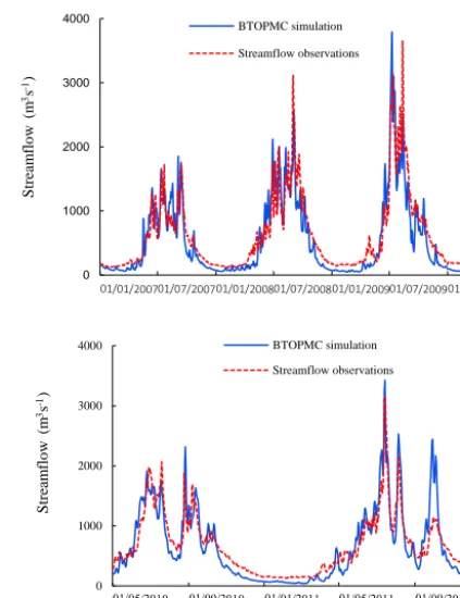
The performance of the multi-model ensemble simulations in both the calibration and validation periods are shown in Fig. 6. From the simulations, it can be seen that the BPNN multi-model ensemble greatly improves the results of a sin-gle member. The BPNN multi-model ensemble adequately reproduces the observed daily streamflow series, withENS values of 0.95 and 0.90 during the calibration and valida-tion periods, respectively. TheENSof the simulation in the ensemble model is satisfactory, and it reproduces the ob-served hydrographs well. The fitting of the flow process in the BPNN multi-model ensemble is clearly better than that of a single member, especially for the relatively low flow pe-riod (from November to April). Moreover, the simulation ac-curacy of the ensemble model for peak flows is also much higher than that of a single model.
5 Conclusions
0 1000 2000 3000
4000 BP Ensemble simulation
Streamflow observations
0 1000 2000 3000 4000
BP Ensemble simulation Streamflow observations
S
tr
ea
m
fl
o
w
(
m
s
)
3
-1
S
tr
ea
m
fl
o
w
(
m
s
)
3
-1
Figure 6.BP ensemble simulated streamflow for the basin in both the calibration and validation periods.
multi-model ensemble takes into account the accuracy of each model, maximizes the use of model information, and has higher precision and stability. The multi-model simula-tion results are more consistent with the observasimula-tions, espe-cially in the low flow and peak flow periods. Multi-model ensemble simulation should become an important direction in hydrological simulation research.
Data availability. The raw data required to reproduce these find-ings are available to download through URLs provided in Sect. 2.2. The processed data required to reproduce these findings cannot be shared at this time as the data also forms part of an ongoing study.
Competing interests. The authors declare that they have no
con-flict of interest.
Special issue statement. This article is part of the special issue “Innovative water resources management – understanding and bal-ancing interactions between humankind and nature”. It is a result of the 8th International Water Resources Management Conference of ICWRS, Beijing, China, 13–15 June 2018.
Acknowledgements. This research was supported by the
National Key Technology Research and Development Program of China (Grant No. 2016YFC0401308), the National Natural Science Foundation of China (Grant Nos. 41671018, 51779007) and Fundamental Research Funds for the Central Universities. Edited by: Yangbo Chen
Reviewed by: two anonymous referees
References
Ajami, N., Duan, Q., and Sorooshian, S.: An integrated hy-drologic Bayesian multimodel combination framework: Con-fronting input, parameter, and model structural uncertainty in hydrologic prediction, Water Resour. Res., 43, W014031, https://doi.org/10.1029/2005WR004745, 2007.
Arnold, J., Srinivasan, R., Muttiah, S., and Williams, J.: Large area hydrologic modeling and assessment – Part 1: Model develop-ment, J. Am. Water Resour. As., 34, 73–89, 1998.
Beven, K. and Binley, A.: The future of distributed models: Model calibration and uncertainty prediction, Hydrol. Process., 6, 279– 298, 1992.
Devineni, N., Sankarasubramanian, A., and Ghosh, S.: Multi-model ensembles of streamflow forecasts: Role of predictor state in developing optimal combinations, Water Resour. Res., 44, W094049, https://doi.org/10.1029/2006WR005855, 2008. Devineni, N., Sankarasubramanian, A., and Ghosh, S.: Multi-model
ensemble hydrologic prediction using Bayesian model averag-ing, Adv. Water Resour., 30, 1371–1386, 2007.
Hu, T., Lam, K., and Ng, S.: A modified neural network for improv-ing river flow prediction, Hydrol. Sci. J., 50, 299–318, 2005. Liang, X., Lettenmaier, D. P., Wood, E., and Burges, S.: A
sim-ple hydrologically based model of land surface water and energy fluxes for general circulation models, J. Geophys. Res.-Atmos., 99, 14415–14428, 1994.
Liang, X., Xie, Z., and Huang, M.: A new parameterization for surface and groundwater interactions and its impact on water budgets with the variable infiltration capacity (VIC) land surface model, J. Geophys. Res.-Atmos., 108, 8613, https://doi.org/10.1029/2002JD003090, 2003.
Najafi, M. R. and Moradkhani, H.: Ensemble Combination of Sea-sonal Streamflow Forecasts, J. Hydrol. Eng., 21, 040150431, https://doi.org/10.1061/(ASCE)HE.1943-5584.0001250, 2016. Razavi, T. and Coulibaly, P.: Improving streamflow estimation in
ungauged basins using a multi-modelling approach, Hydrol. Sci. J., 61, 2668–2679, 2016.
Saxton, K. R. W.: Soil water characteristic estimates by texture an-dorganic matter for hydrological solutions, Soil Sci. Soc. Am. J., 70, 1569–1578, 2006.
Takeuchi, K., Hapuarachchi, P., Zhou, M., Ishidaira, H., and Magome, J.: A BTOP model to extend TOPMODEL for dis-tributed hydrological simulation of large basins, Hydrol. Pro-cess., 22, 3236–3251, 2008.
Wang, J., Shi, P., Jiang, P., Hu, J., Qu, S., Chen, X., Chen, Y., Dai, Y., and Xiao, Z.: Application of BP Neural Network Algorithm in Traditional Hydrological Model for Flood Forecasting, Water, 9, 48, https://doi.org/10.3390/w9010048, 2017.
predicting river monthly flows, Hydrol. Sci. J., 58, 374–389, 2013.
Yaseen, Z., El-Shafie, A., Jaafar, O., Afan, H., and Sayl, M.: Artifi-cial intelligence based models for stream-flow forecasting: 2000– 2015, J. Hydrol., 530, 829–844, 2015.