Forecasting Natural Events using Axonal Delay
David Reid Liverpool Hope University
Liverpool L16 9JD [email protected]
Hissam Tawfik Leeds Beckett University
Leeds LS1 3HE
Abir Jaafar Hussain Liverpool John Moores University
Liverpool L3 3AF [email protected]
Rozaida Ghazali
Universiti Tun Hussein Onn Malaysia Malaysia
Abstract—The ability to forecast natural phenomena relies on understanding causality. By definition this understanding must include a temporal component. In this paper, we consider the ability of an emerging class of neural network, which encode temporal information into the network, to perform the difficult task of Natural Event Forecasting. The Axonal Delay Network (ADN) models axonal delay in order to make predictions about sunspot activity, the Auroral Electrojet (AE) index and daily temperatures during a heatwave. The performance of this network is benchmarked against older types of neural networks; including the Multi-Layer Perceptron (MLP) network and Functional Link Neural Network (FLNN). The results indicate that the inherent temporal characteristics of the Axonal Delay Network make it well suited to the processing and prediction of natural phenomena.
Keywords—axonal delay, spiking neural network, natural event forecasting
I. INTRODUCTION
Natural event prediction is difficult; this is due to the nonlinearity and non-stationary properties of the data. Natural events such as earthquakes, weather and sunspot data sets are complex in nature and often exhibit chaotic behaviour. For example, earthquake data may be complicated from data originating from other sources. These may be from as other seismic patterns, electromagnetic fields, weather conditions, hydrogen gas content of soil, water level in wells as well as animal behavior [1]. The complexity of the interrelationship between these sets of data means that despite massive increases in computational power it is still notoriously difficult to predict when an earthquake will occur as well as the location and severity of that earthquake.
Similarly, predictions of weather signals such as rainfall are crucial and important for reservoir operations to preventing flooding. Rainfall rates are a key indicator of lead-time of
river flow forecast, this in turn is useful for reservoir control [2].
Using a conventional approach to model natural events is problematic, as they often do not inherently encode temporal information nor have the facilities to account for complex interaction of different types of phenomena [3].
Natural events often have inherent temporal dynamics that are highly complex and present significant challenge to time-series predication models. For our purposes, time-time-series prediction can be defined as the estimation of future values of the series based on some past-observed values [4]. A predictor is able to discover approximate functions between the input and the output values [5], [6]. This function can be used to forecast the future value.
In order to generate good simulation prediction, two processes are required: pre-processing of the natural data sets using various techniques such as Moving Average and Singular Spectrum Analysis, followed by the application of appropriate prediction techniques (such as statistical and machine learning methods [2]).
It is increasingly being recognized that to predict natural events with any degree of accuracy that time series data has to be utilized. This has often formed the basis of new, testable, prediction models. Such models exist in order to discover functions or relationships between the past observations in order to construct more accurate predictions [6], [7].
techniques are consider the relations between the signal elements to be highly correlated and hence assume that the previous observation of the data series can be used to predict future observations in a simpleminded manner. They assume past and future events have a one-to-one correlation [8]. The Moving Average (MA) is a little more complex in that it measures the mean of a set of previous observations in the time series, the mean values are then used to predict future observations of the time series [9]. The Auto-Regressive Moving Average model (ARMA) is based on both the AR and MA [10]. In all of these models however the time series is assumed to be stationary.
For non-stationary time series data, Auto-Regressive Integrated Moving Average (ARIMA) can be used for time series prediction [11]. The model extend the ARMA, with the signals being integrated before creating forecasts. The integration means that the forecasted values are expressed with reference to the values of the input data. Once this step is completed ARIMA model assumes that the data can be stationary [12]. The model has been considered the basis for time series analysis and has been widely used in financial predictions [13], [14].
However, despite the wide adoption of these traditional forecasting models, their ability to model time series is limited [4], [15]. They assume that the relations between data in time series are linear, and prediction takes place under stationary conditions. In nature as relations in most time series are complex and nonlinear traditional linear prediction methods are poor at capturing nuances and are therefore are too simplistic for accurate prediction [16]. As such there is a growing need to find more robust and powerful prediction methods that can overcome the traditional prediction models’ limitations. Consequently, the use of nonlinear and machine learning methods as predictors is in great demand.
This paper investigates the use of a type of neural network that has temporal processing as a core function. A fundamental operation of a Spiking Neural Network (SNN) is to take into account when an event occurs and to trigger events at specific times. This cascading of events leads to strengthening or weakening of the simulated synapses between neurons in this network. As such the role of Axonal Delay is fundamental in the mediation of learning in such a network. It is these networks, and specifically the role of Axonal Delay in learning that this paper examines.
II. ARTIFICIAL NEURAL NETWORKS FOR TIME SERIES FORECASTING
When applied to time series prediction Artificial Neural Networks (ANNs) exhibit features of robustness and fault-tolerance and can overcome the limitations of statistical approaches. ANNs are able to generalise the model to predict new data and can thereby increase the probability of producing correct predictions [4]. It is rare to have pristine real-world sets of time series data available for processing [16].
Therefore, the predictor model must have the ability to discover the correct internal presentation and capture the hidden pattern of time series [5]. ANNs have been seen as a good mechanism to process messy time series data. To do this ANNs need to be designed in such a way that the input data presented to the neural network are drawn from a number of sequential previous inputs and the output is the value of a future step in time. The ANNs most widely used as time series predictors are MLP [17], and the Elman Neural Network (ERNN) [18], [19]. A number of studies have proved that using ANN in modelling and predicting time series can produce favourable results.
However, there are a number of problems associated with the use of these types of neural networks in time series prediction. Different neural networks algorithms can produce different results when trained and tested on the same data set. For any given type of neural networks, the network can be sensitive to the network size and the size of the data set. Neural networks can suffer from overfitting and as a result the network architecture, learning parameters and training data have to be selected carefully in order to achieve good generalization. This is critical when using the network for time series prediction. Above all, the highly complex nature of natural event time series data can easily thwart the predicative capabilities of such ANNs.
Unlike the older class of ANNs, Spiking Neural Networks (SNNs) have shown that they are particularly robust in detecting and classifying complex real world data. They are particularly well suited to model time-series complexity because an inherent characteristic of these networks, spike timing, can be very naturally used to encode data [20], [21], [22].
SNNs are inherently suited to manage highly non-linear and temporal based input data that traditional neural networks struggle with. A relatively small number of researchers have applied Spiking Neural Network systems in order to classify and predict natural time series data. Typically, such networks involve choosing a particular feature set, which are then used to explicitly analyse and classify data. It is proposed in this paper that the explicit engineering of the temporal aspects of events in nature into data for the SNNs, and the fine control of Axonal Delay, make it more suited to time series analysis of natural events than are older types of neural networks [22], [23], [24].
III. SPIKING NEURAL NETWORKS AND AXONAL DELAYS
A. Background
synaptic plasticity linked with Axonal Delay form an intricate network of reciprocally connected areas to provide a finely balanced framework for learning.
SNNs take into account the inherent temporal nature of the brain and as such are far more capable in processing the nuances of complex temporal data than traditional ANNs [26]. Two types of SNNs models dominate. The “Leaky Integrate and Fire” (LIF) model [22] and the Izhikevich model [24], [27]. As the later model can simulate a much wider array of spiking behavoir than the former and is relatively easy to embed Axonal Delay into its function, it was this type of SNN that was used for the work presented in this paper.
B. Izhikevich Model
The Izhikevich model can be defined by the following two differential equations:
(1) Where v is voltage potential and u is the membrane recovery and W is the weighted input.
When v exceeds a threshold value both v and u are reset as follows:
(2)
a and b are recovery parameters. c is the target value for v
after a spike. d is a constant value added to u after a spike.
C. Learning
The learning rule most commonly used derived from Hebbian learning called Spike Time Dependent Plasticity (STDP) [26], [27]. STDP uses the spike time difference between input and output spikes to adjust synapse connection strength. Synapses increase if a pre-synaptic spike arrives just before the postsynaptic neuron is activated, but are weakened if they occur afterwards [20], [21], [28].
Thus the weight change of a synapse from a pre-synaptic neuron j depends on the timing between pre-synaptic spike arrivals and postsynaptic spike departures from neuron i. Thus if we have:
where f is pre-synaptic spike count at time t, and is the postsynaptic spike count at time t .
The weight change can be calculated as:
(3) The W function is:
for x >0
for x<0
(4) A+ and A- are values dependent on the current synaptic weight and and are time constants.
D. Encoding Axonal Delay
SDTP rewards tightly coupled time dependent cause and effect. Learning is a function of associating the temporal sequence of spiking events. By chaining these events together a temporal pattern can be encoded.
By doing this a large number of spiking patterns, or trains, are processed by a relatively modest number of neurons. This cascade of spiking activity means that neurons in such a system are associated to each other by axonal delay. Neuronal chains of firing patterns that may spontaneously emerge in such a network are called gamma rhythms [29]. Generation of gamma rhythms are an indication that groups of neurons are learning to fire, and hence wire, together.
The recognition of not only where, but when, an event occurs gives SNNs the capability to rapidly recognize complex temporal patterns.
Axonal Delay and STDP learning may be important constructs to use in the effort to make sense of complex natural time series based phenomena. As such, they have the potential to produce better predictive performance compared to traditional paradigms.
IV. EXPERIMENTS AND RESULTS
A. Axonal Delay Network (ADN)
A key feature of the approach we adopt for this paper is that training data can be presented to the network with minimal preprocessing. The only requirement is that the data is scaled in order to map values to the available number of neurons. This is done to reduce the range difference in the data, to process outliers, and to accommodate the limits of the network’s transfer function. The calculation for the standard minimum and maximum normalization method used is as follows:
(5) where x’ is the normalized value, x is the original value, min
1 and max1 are the respective minimum and maximum values of all observations, and min2 and max2 refer to the desired minimum and maximum of the new scaled series.
the time series values onto distinct neurons. This aided both encoding and decoding of the data and eased processing. It also made it easy to see when particular neurons are firing.
Training of the network consisted of scaling and presenting the scaled values to the network via the value W in equation (1).
An abstract perspective for the entire process is presented in the following snippet of pseudocode.
As can be seen above, the process follows a process of scaling, setting the thalamic input (W) of the mapped neuron, firing, learning, comparing, extracting, and finally extrapolating results.
Three different training architectures were applied: randomly connected neurons, bands of connected neurons and focused neural connection.
It was found that focused single neurons connected to afferent neurons (updated with each training cycle) were 4-5 times faster to train than the other methods. During training the system periodically entered bursts of activity that indicated that afferent neurons were being activated, in a manner suggesting a gamma cycle.
Neurons firing at the midpoint of the dataset were labelled as “anchor” neurons. These are neurons that have been influenced by, or will influence, other significant neurons in a chain of activity. The network then looked for all possible pre-synaptic firing patterns in the previous 200 afferent neuron values that where similar to the previous 200 real data values (a tolerance of ±5ms was given). These acted as possible “candidate” paths of firing activity.
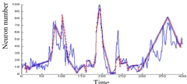
The candidate path that was closest in terms of Euclidean distance from the real data was then chosen. This forms the basis of the forecast. The probability of the continuation of firing of the candidate path to the efferent neurons provides the prediction. In other words the most likely to fire neurons in the 201st, 202nd 203rd , up to 400th time series spike time where selected. The resultant spike train/path is shown in Figure 1.
Fig. 1. The closest firing path of the sunspot times series. The forecast was based on different combinations of possible neuronal paths. Each candidate path was ranked according to when neurons fired and which afferent neurons influenced them. The candidate path through the network that most closely resembles the real time series data was deemed to be the best approximate forecast.
B. The Natural Events Time Series
To test this technique three natural signals were used for our experiments; the mean value of the Auroral Electrojet index (AE) index, daily temperatures during a heatwave and the Sunspot Number time series.
The AE index can be determined from weather stations positioned in high latitude areas. In these stations, the north-south magnetic perturbations are calculated as a function of time and the superposition of the measured data determines two components, the maximum negative and the maximum positive magnetic perturbations. The difference between the two components is called the AE index [30].
(a)
(b) Fig. 2. (a) The mean value of the AE index time series. (b) The correlogram of the mean value of the AE index signal.
Time
Day
A
ut
oc
or
re
la
tio
n
co
ef
fi
ci
en
ts
N
eu
ro
n
nu
m
be
r
M
ea
n
V
al
ue
o
f
A
E
I
nd
To investigate the nonstationary properties of the AE signal, the correlogram is determined in Figure 2 (b). As the autocorrelation coefficients drop to zero for large values of the lag this can conclude the nonstationary properties of the signal. Figure 2 (b) also shows that the signal has periodicities for every 5000 lags.
The second natural time series used in our experiments is the Oklahoma City US daily heat wave temperatures. This data was obtained from the National Oceanic and Atmosphere Administration. The signal is collected for five months from May to September 2012 as shown in Figure 3 (a). Heat wave temperatures are in Fahrenheit and used for the pattern prediction. As indicated in Figure 3 (b), the correlogram goes to zero for a large value of the lag showing nonstationary properties with no periodicity.
0 25 50 75 100 125 150
60 70 80 90 100 110
H
ae
tw
av
e
Te
m
p
Fahrenheit
(a) Lag(b)
Fig 3. (a) The heatwave temperature time series. (b) The correlogram of the signal.
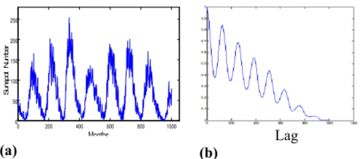
The final natural event times series considered was the Sunspot Number time series.
Various solar indices can be used to express the activity of the sun. However, the International Sunspot Number (ISN) is one of the key indicators since the data is exceptionally lengthy and collected over a number of years. Research studies show that predicting sunspot activity data is important for spacecraft and communication [31]. Figure 4 (a) shows the sunspot time series meanwhile Figure 4 (b) shows the correlogram of the signal. Similar to the AE and heat wave signals, the Sunspot signal corrologram also drops to zero for large value of the lag showing nonstationary properties of the signal.
0 200 400 600 800 1000
0 50 100 150 200 250
Months
Su
ns
po
t
N
um
be
r
(a) Lag(b)
Fig. 4. (a) The sunspot number time series from the year 1930 to 2013. (b) The correlogram of the signal.
C. Experimental Testing
In these experiments we benchmarked the performance of the spiking neural network with multilayer perceptron (MLP) Neural network and the functional link (FLNN) neural network [32], [33], [34]. The normalised mean square of the error (NMSE) and the signal to noise ratio (SNR) matrices are used as quality measures for our experiments and are calculated as in Table 1.
The data sets are segregated in time order with earlier period of data are used for training, while later period are used for testing. This will help us to understand the relationship exist between past, present and future data. For the MLP and FLNN each signal was divided into three data sets which are training, validation and the out-of-sample with 25%, 25%, and 50% of the entire data, respectively. For the proposed AND, only the last data set is used.
NMSE SNR
Table 1. Performance Metrics
The ADN was benchmarked with the MLP and the FLNN trained with the incremental backpropagation learning algorithm.
In our experiments, average values over 5 trials are used. The learning rates and the momentum term were experimentally selected.
Mean Value of the AE index
MLP FLNN ADN
NMSE 0.175805 0.133661 0.0029796
SNR (dB) 28.3 29.45 39.9127
Sunspot number
MLP FLNN ADN
NMSE 0.1319 0.1366 0.005011
SNR (dB) 25.16 25.01 32.4729
Heatwave Signal MLP FLNN ADN
NSME 0.4938 0.4903 0.075593
SNR 18.12 18.15 22.9191
Table 2. The average simulation results over 5 trials using the benchmarked Neural Networks Structures.
V. CONCLUSION
In this paper, we have considered a specific type of spiking neural networks, called Axonal Delay Network, to investigate the prediction of natural event time series data, with the aim to investigate the temporal characteristics of the Spiking Neural Network model.
The proposed Spiking Neural Network model utilised Izhikevich neural architecture with Axonal Delays, directly encoding the time series data into the model in such a way as to try to preserve valuable temporal predictive indicators. Experiments using our ADN showed that it outperforms traditional, rate-encoded, neural networks, namely Multi-Layer Perceptrons (MLP) and a higher order Functional Link Neural Network (FLNN). This was validated using three time series datasets: Mean Value of the Auroral Electrojet (AE) index, daily temperatures during a heatwave and a Sunspots Number dataset. Using the Normalised Mean Squared Error and the Signal to Noise Ratio showed that the ADN has improved performance. Future work includes exploring the applicability of ADN for long term prediction, exploring the effects of parameter tuning of the ADN on its performance, the potential incorporation of higher order terms in the spiking neural network.
REFERENCES
[1] M. Moustra, M. Avraamides, C. Christodoulou, “Artificial neural networks for earthquake prediction using time series magnitude data or Seismic Electric Signals” Expert Systems with Applications 38, 15032– 15039. 2011
[2] C.L. Wu, K.W. Chau,“Prediction of rainfall time series using modular soft computing methods”, Engineering Applications of Artificial Intelligence 26, 997–1007, 2013
[3] A. Knoblauch, G. Palm, F. T. Sommer, “Memory capacities for synaptic and structural plasticity”, Neural Computation 22 (2), 289-341, 2010 [4] J. L. Herrera, “Time Series Prediction Using Inductive Reasoning
Techniques”, Instituto de Organizacion y Control de Sistemas Industriales, 1999
[5] V. Petridis, A. Kehagias, L. Petrou, et al, “A Bayesian Multiple Models Combination Method for Time Series”, Journal of Intelligent and Robotic Systems, 31, pp.69–89, 2001
[6] L. J. Elman, “Finding Structure in Time”, Cognitive Science 14, pp. 179-211, 1990
[7] R. Rape, D. Fefer, and J. Drnovsek, "Time series prediction with neural networks: a case of two examples," IEEE Instrumentation and measurement technology conference, Hammamatsu, Shizuoka, Japan, 10-12 May 1994, pp. 145-148,1994.
[8] C. L Dunis, M. Williams, “Applications of Advanced Regression Analysis for Trading and Investment”, Quantative Methods for Trading and Investment, John Wiley & Sons, New York, pp 1-40, 2003 [9] A. Sfetsos, “A comparison of various forecasting techniques applied to
mean hourly wind speed time series”, Renewable Energy, 21(1), pp.23– 35, 2000
[10] S. Porter-hudak, “An Application of the Seasonal Fractionally Differenced Model to the Monetary Aggregates”, Journal of the American Statistical Association, 85(410), pp.338–344, 1990
[11] S. E. Alnaa, F. Ahiakpor, “ARIMA (autoregressive integrated moving average) approach to predicting inflation in Ghana”, Journal of Economics and International Finance, 3(May), pp.328–336, 2011
[12] S. Ho, M. Xie, T. N. Goh, “A comparative study of neural network and Box-Jenkins ARIMA modeling in time series prediction”, Computers & Industrial Engineering, 42(2-4), pp.371–375, 2002
[13] S. Yümlü, F. S. Gürgen, N. Okay, N., “A comparison of global, recurrent and smoothed-piecewise neural models for Istanbul stock exchange (ISE) prediction”, Pattern Recognition Letters, 26(13), pp.2093–2103, 2005
[14] R. Ghazali, A. Hussain, N. Nawi, B. Mohamad, “Non-stationary and stationary prediction of financial time series using dynamic ridge polynomial neural network”. Neurocomputing, 72(10-12), pp.2359– 2367, 2009
[15] G. E. P. Box, G. W. Jenkins, G. C. Reinsel, “Time Series Analysis -Forecasting and Control (3rd edition)”, Englewood Cliffs, NJ:Prentice-Hall, 1994
[16] F. Castiglione, “Forecasting price increments using an artificial Neural Network”, Complex Dynamics in Economics - a Special Issue of Advances in Complex Systems, 4(1): 45-56, Hermes-Oxford, 2001 [17] L. J. Cao, F. E. H. Tay, “Support Vector Machine with Adaptive
Parameters in Financial time Series Forecasting”, IEEE Transactions on Neural Networks, 14(6), pp.1506–1518, 2003
[18] M. W. Pedersen, “Optimization of Recurrent Neural Networks for Time Series Modeling”. PhD thesis. Technical University of Denmark, 1997 [19] J. Conner and L. Atlas “Recurrent neural networks and time series
prediction”, IEEE International Joint conference on Neural networks, New York, USA, pp. I 301- I 306, 1991.
[20] A. Hodgkin, and A. Huxley, “A quantitative description of membrane current and its application to conduction and excitation in nerve,” J. Physiol., vol. 117, pp. 500–544, 1952.
[21] M. Abeles , “Corticonics: Neural circuits of the cerebral cortex,” Cambridge University Press, New-York, 1991.
[22] W. Maass, “ Networks of Spiking Neurons: The Third Generation of Neural Network Models,” Neural Networks, vol. 10, no. 9, Elsevier Publishing, pp. 1659-1671, Dec. 1997.
[23] W. Maass, and C. M. Bishop, “ Pulsed Neural Networks,” MIT press, ISBN 0-262-13350-4, 1998.
[24] E. M. Izhikevich, “Simple model of spiking neurons,” IEEE Transactions on Neural Networks, vol. 14 , no. 6 ,pp. 1569 – 1572, 2003.
[25] W. B. Levy, and O. Steward, "Temporal contiguity requirements for long-term associative potentiation/depression in the hippocampus,"
Neuroscience, vol. 8, no. 4, pp. 791-7, Apr. 1983.
[26] R. Legenstein, C. Naeger, and W. Maass, “What can a Neuron Learn with Spike-Timing-Dependent-Plasticty,” Journal of Neural Computation, vol. 17, no. 11, pp. 2337-2382, 2005.
[27] E. M. Izhikevich, “Polychronization: Computation with Spikes,” Journal of Neural Computation, vol. 18, no. 2, pp. 245-282, 2006.
[28] H. Markram, J. Lübke, M. Frotscher, and B. Sakmann, "Regulation of synaptic efficacy by coincidence of postsynaptic APs and EPSPs,"
Science 275 (5297), pp. 213–5, Jan. 1997.
[29] J. V. Arthur, and K. A. Boahen, ”Synchrony in Silicon: The Gamma Rhythm,” IEEE Transactions on Neural Networks, vol. 18, no. 6, 2007. [30] NOAA. National Ocean and Atmosphere Administration, National
Weather Service - Norman, Oklahoma, http://www.srh.noaa.gov/oun/? n=climate-okc-heatwave, 2012.
[31] J. Makhoul “Linear prediction: A tutorial review,” Proceedings of the IEEE, 63(4), pp. 561-580, 1975.
[32] J. Tang and X. Zhang “Prediction of smoothed monthly mean sunspot number based on chaos theory”, Acta physica sinica, 61 ( 16), Article Number: 169601, 2012.
[33] R. Durbin, D. E. and Rumelhart, “Product Units: A Computationally Powerful and Biologically Plausible Extension to Back-propagation Networks,” Neural Computation, vol. 1, pp. 133-142, 1989.