Development of Robot Navigation System with Collision Free Path Planning Algorithm

(1)

http://www.sciencepublishinggroup.com/j/mlr doi: 10.11648/j.mlr.20180303.12

ISSN: 2637-5672 (Print); ISSN: 2637-5680 (Online)

Development of Robot Navigation System with Collision

Free Path Planning Algorithm

Htun Myint

Department of Electronic Engineering, Technological University (Panglong), Panglong, Myanmar

Email address:

To cite this article:

Htun Myint. Development of Robot Navigation System with Collision Free Path Planning Algorithm. Machine Learning Research. Vol. 3, No. 3, 2018, pp. 60-68. doi: 10.11648/j.mlr.20180303.12

Received: August 3, 2018; Accepted: September 6, 2018; Published: October 12, 2018

Abstract:

Mobile robots have been successfully used in many fields due to their abilities to perform difficult tasks in hazardous environments, such as robot rescuing, space exploring and their various promising applications in the daily lives. Robot path planning is a key issue in robot navigation which is a kernel part in mobile robot technology. Robot path planning is to generate a collision-free path in an environment while satisfying some optimization criteria. Mobile robot path planning is a nondeterministic polynomial time (NP) problem, traditional optimization methods are not very effective to it, which are easy to plunge into local minimum. In this research work, an evolutionary algorithm to solve the robot path planning problem is devised. A method of robot path planning in partially unknown environments based on A star (A*) algorithm was proposed. The proposed algorithm allows a mobile robot to navigate through static obstacles and finds its path in order to reach from its initial position to the target without collision. In addition, the environment is partially unknown for the robot due to the limit detection range of its sensors. The robot processor updates its information during the motion. The simulations are performed in different static environments, and the results show that the robot reaches its target with colliding free obstacles. The optimal path is generated with this method when the robot reaches its target. The simulation results are developed by MATLAB environments.

Keywords:

Collision Free Path, Robot Navigation, MATLAB, A Star, Path Planning Algorithm

1. Introduction

Robotic is known as a new revolution to the entity of beings that varies according to its uses. In modern day environments, robotics and automation are involved in almost every industrial activity and conveniently improve the efficiency, productivity and reliability of a system. Robotics is also implemented in medical practice, construction, outer-space exploration, household assistance, mobile transportation and quite recently, underwater exploration. Robots have many uses in the military, industry, health care services, and neighborhood homes. Robots categorized as unmanned ground, marine, and aerial vehicles are normally found in the military. In industry, robots are commonly used on assembly lines in automotive and food processing plants. These robots are usually in the category of machine vision and used to assemble products and/or detect defects in the products. In health care, robots are now used to assist during surgical procedures. Robotic devices are also starting to be used to assist elderly people, particularly in Japan. It could also be

(2)

Machine Learning Research 2018; 3(3): 60-68 61

New technology such as autonomous vehicle systems may also be able to utilize such algorithms which are fail-safe. The robotic platform design is not an issue anymore. Whether the robot will serve the military or be a part of the civilian workforce, the platform will be designed to support the required application. For a vehicle to travel longer distances in a shorter amount of time, it will be necessary to eliminate the long delay caused by communications traveling across the great distance between source and destination. One possibility involves breaking the traditional laws of physics and finding a way to communicate faster than the speed of vehicle. An easier approach involves eliminating the need for such frequent communications. This implies that any such vehicle will have to be able to perform two tasks on its own [9-13].

(1) Determine the three-dimensional layout, or map, of the surrounding terrain by use of photographs taken from multiple locations

(2) Determine a path across this map to reach the intended destination.

The main objective of this project is to create and develop a Path Planning Mobile Robot able to avoid obstacles in its path and reach a target designated position from its starting point. A study on obstacle avoidance using A* algorithm, path planning. The overall system block diagram is illustrated in Figure 1.

Figure 1. System Block Diagram.

**2. A* Path Finding Algorithm**

A real challenge for an agent in real time games is to find the route from the start node to the goal node in presence of other agents and obstacles. In the presence of obstacles, the path moves around the obstacle and reaches the goal. This path should be of minimum cost or in other words it should be the shortest possible distance. A* is a shortest path finding algorithm that uses informed search technique to find the least-cost path from the start node to the goal node. The classic representation of the A* algorithm is as follow:

f(x) = g(x) + h(x)

f(x): is called the distance-plus-cost heuristic function (or simply F cost) and it is the sum of path-cost function g(x) and heuristic function h(x).

g(x): the path-cost function (or simply G cost) is the actual total cost of the path to reach the current node x from the start node.

h(x): is the estimated cost (or simply H cost) of the path from current node x to the goal node. An estimate is made that

tells how far the goal node is from the current node x. h(x) must be an admissible heuristic estimate. A heuristic function is said to be admissible if the cost of path estimated by it never exceeds the lowest-cost path. Since h(x) is part of f(x), f(x) is dependable on h(x) for the lowest cost of path. It means when h(x) is admissible, A* algorithm is guaranteed to give the shortest path if one exists. Therefore, h(x) must not overestimate the cost. The cost is measured by meter (m). There are many different heuristic functions used for the grid maps. Some famous heuristics are Manhattan distance, diagonal distance, Euclidean distance. Manhattan distance to estimate h(x) because it works better on squared grids is used. It is the direct distance from current node to the goal node without considering obstacles in the path. In this way h(x) is giving us the lowest possible cost to reach the goal node [14-17].

**3. Linking Functions for A* Algorithm**

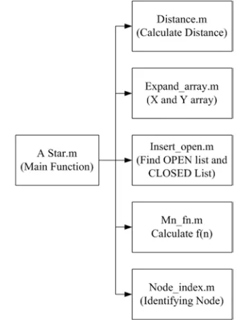
The implementation of A* algorithm for mobile robot path planning system is developed by linking the main and sub-functions of MATLAB script. There are only six functions for function linking system.

Figure 2. Block Diagram of Linking System for MATLAB Function.

They are A Star.m for main function and Distance.m for distance calculation, Expand_array.m for X and Y array specifying, Insert_open.m for finding the OPEN and CLOSED list, Mn_fn.m for f(n) calculation and Node_index.m for identifying node. The block diagram of linking system for MATLAB function is shown in Figure 2.

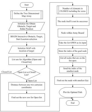
**4. Overall Flowchart of A* Algorithm**

(3)

Figure 3. Overall Flowchart of Mobile Robot Path Planning.

5. Development of Main Function for A*

Path Planning Algorithm

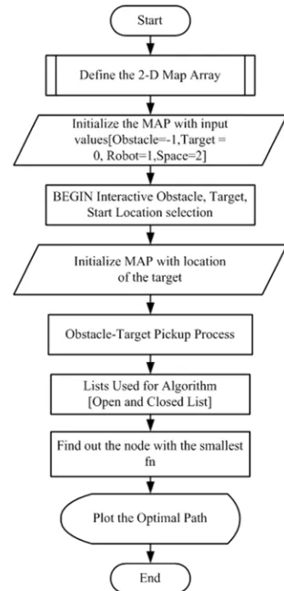
According to the A* algorithm the path planning algorithm is accomplished with the help of MATLAB to find the optimal path of mobile robot. There are four main steps to find the optimal path for mobile robot. They are defining the 2-D map array on the work space, specifying the source, target and obstacle locations with the help of mouse button, finding the node with the smallest f(n), and plotting the optimal path on the work space. All distances are measured by SI unit (Meter). First, the MATLAB codes are implemented according to the defining the 2-D map array on the work space as follows:

MAX_X=10; MAX_Y=10; MAX_VAL=10;

The values of MAX_X, MAX_Y, and MAX_VAL are changed by the necessary of work space specification for mobile robot path planning. This array stores the coordinates of the map and the Objects in each coordinate by using the below code.

MAP=2*(ones(MAX_X,MAX_Y));

And the position of Obstacle, Target and Robot have to be initialized on the MAP with input values as Obstacle=-1, Target = 0, Robot=1, Space=2. The program is begun with the interactive Obstacle, Target, Start location selection by commanding the following message boxes on the work space. h=msgbox('Please Select the Target using the Left Mouse button');

h=msgbox('Select Obstacles using the Left Mouse button, to select the last obstacle use the Right button');

h=msgbox('Please Select the Vehicle initial position using the Left Mouse button');

After inputting the information on these message box, the position of Obstacle, Target, Start are displayed on the work space and waiting the algorithm to find the optimal path.

Then the lists used for algorithm to calculate the distance travels of mobile robot with OPEN and CLOSED list on the work space is implemented by using the specified MATLAB codes.

(4)

for i=1:MAX_X for j=1:MAX_Y if(MAP(i,j) == -1) CLOSED(k,1)=i; CLOSED(k,2)=j; k=k+1;

end end end

After counting the CLOSED list on the work space, the matrix size of CLOSED list to find the path distance is developed by following the below instruction.

CLOSED_COUNT=size(CLOSED,1);

And then the starting node as the first node is set to find the next distance by accumulating the node location with the help of the following instructions.

xNode=xval; yNode=yval; OPEN_COUNT=1; path_cost=0;

goal_distance=distance(xNode,yNode,xTarget,yTarget); OPEN(OPEN_COUNT,:)=insert_open(xNode,yNode,xNo de,yNode,path_cost,goal_distance,goal_distance);

OPEN(OPEN_COUNT,1)=0;

CLOSED_COUNT=CLOSED_COUNT+1; CLOSED(CLOSED_COUNT,1)=xNode; CLOSED(CLOSED_COUNT,2)=yNode; NoPath=1;

According to the specifying the OPEN and CLOSED list on the work space, the A* algorithm is started by expanding the array format. There are two main stages for counting condition. The first one is finding the OPEN count and the second one is updating the OPEN count by following the for loop expressions.

for i=1:exp_count flag=0;

for j=1:OPEN_COUNT

if(exp_array(i,1) == OPEN(j,2) && exp_array(i,2) == OPEN(j,3) )

OPEN(j,8)=min(OPEN(j,8),exp_array(i,5)); if OPEN(j,8)== exp_array(i,5) OPEN(j,4)=xNode;

OPEN(j,5)=yNode; OPEN(j,6)=exp_array(i,3); OPEN(j,7)=exp_array(i,4); end;

flag=1; end; end; if flag == 0

OPEN_COUNT = OPEN_COUNT+1;

The node with the smallest f(n) is analyzed by applying the following MATLAB codes.

index_min_node =

min_fn(OPEN,OPEN_COUNT,xTarget,yTarget);

The xNode and yNode to the node with minimum f(n) is set to update the cost of reaching the parent node.

xNode=OPEN(index_min_node,2); yNode=OPEN(index_min_node,3); path_cost=OPEN(index_min_node,6);

After finding the cost of reaching the parent node, the node to list CLOSED is moved by using the following codes.

CLOSED_COUNT=CLOSED_COUNT+1; CLOSED(CLOSED_COUNT,1)=xNode; CLOSED(CLOSED_COUNT,2)=yNode; OPEN(index_min_node,1)=0;

Once the algorithm has run the optimal path is generated by starting off at the last node (if it is the target node) and then identifying its parent node until it reaches the start node. This is the optimal path of the mobile robot. The following instructions are appropriated to find the optimal path.

i=size(CLOSED,1); Optimal_path=[]; xval=CLOSED(i,1); yval=CLOSED(i,2); i=1;

Optimal_path(i,1)=xval; Optimal_path(i,2)=yval; i=i+1;

Based on the above MATLAB instructions to find the optimal path, the optimal path is plotted on the work space by using the following code.

p=plot(Optimal_path(j,1)+.5,Optimal_path(j,2)+.5,'bo'); The completed MATLAB code is shown in APPENDIX of this dissertation.

(5)

5.1. Development of Distance.m Function

This function calculates the distance between any two Cartesian coordinates. The straight line equation is applied to find the distance along the mobile robot path finding stage. This function is very simple and easy to use the next update distance of target node by using the following MATLAB code.

dist=sqrt((x1-x2)^2 + (y1-y2)^2);

The detailed calculations for path distance are as follows: Let x1=0, y1=0, and the open list can be (2,1)

∴x2=2 and y2=1

dist= x1-x2 2_{+ y1-y2} 2

dist= 0-2 2+ 0-1 2=2.23 meters

5.2. Development of Expanded_Array.m Function

This function takes a node and returns the expanded list of successors, with the calculated f(n) values. The criteria being none of the successors are on the CLOSED list. Number of elements in CLOSED including the zeros matrix is satisfied by using the following MATLAB codes.

exp_array=[]; exp_count=1; c2=size(CLOSED,1);

The node itself is not its successor for node within array bound and to check if a successor is on closed list by using the following MATLAB instructions.

for k= 1:-1:-1 for j= 1:-1:-1 if (k~=j || k~=0) s_x = node_x+k; s_y = node_y+j;

if( (s_x >0 && s_x <=MAX_X) && (s_y >0 && s_y <=MAX_Y))

flag=1; for c1=1:c2

if(s_x == CLOSED(c1,1) && s_y == CLOSED(c1,2))

flag=0; end; end

And the distance or cost of travelling to node is developed with the below code.

exp_array(exp_count,3) =

hn+distance(node_x,node_y,s_x,s_y);

The distance between node and goal and f(n) are analyzed by the following MATLAB instructions.

distance(xTarget,yTarget,s_x,s_y);

exp_array(exp_count,3)+exp_array(exp_count,4);

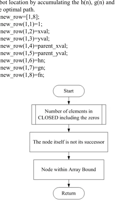
The flowchart of Expanded_array function is illustrated in Figure 5.

5.3. Development of Inset_Open.m Function

This function is to populate the OPEN list by using the following instructions in MATLAB. The new row for mobile robot location by accumulating the h(n), g(n) and f(n) to find the optimal path.

new_row=[1,8]; new_row(1,1)=1; new_row(1,2)=xval; new_row(1,3)=yval; new_row(1,4)=parent_xval; new_row(1,5)=parent_yval; new_row(1,6)=hn;

new_row(1,7)=gn; new_row(1,8)=fn;

Figure 5. Expanded Array Flowchart.

5.4. Development of Node with Minimum f(n)

This function takes the list OPEN as its input and returns the index of the node that has the least cost by applying the following MATLAB code. In this code, the indexes of the goal node are stored and get all nodes that are on the list open.

temp_array=[]; k=1;

flag=0; goal_index=0;

for j=1:OPEN_COUNT if (OPEN(j,1)==1)

temp_array(k,:)=[OPEN(j,:) j];

if (OPEN(j,2)==xTarget && OPEN(j,3)==yTarget) flag=1;

goal_index=j; end;

(6)

Figure 6. Flowchart of Node with Minimum f(n).

One of the successors is the goal node so send this node and it is implemented by the following MATLAB codes. And the index of the smallest node can be sent to the updating stage.

if flag == 1 i_min=goal_index; end

Index of the smallest node in temp array and index of the smallest node in the OPEN array are developed by the following codes.

if size(temp_array ~= 0)

[min_fn,temp_min]=min(temp_array(:,8)); i_min=temp_array(temp_min,9);

else

The flowchart of Node with Minimum f(n) function is demonstrated in Figure 6.

5.5. Development of Node_Index.m Function

This function returns the index of the location of a node in the list OPEN and it can be identified by using the following MATLAB instructions.

i=1;

while(OPEN(i,2) ~= xval || OPEN(i,3) ~= yval ) i=i+1;

end; n_index=i;

5.6. Debugging the A Star Search Algorithm

After implementing the A star search algorithm in the previous chapter, the collision free path planning algorithms is debugged in MATLAB command window. The information window for selecting the target node with the help of mouse button is displayed. This information window is shown in Figure 7.

Figure 7. Information Window for Selecting the Target Node.

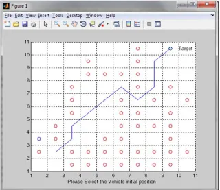
The first simulation result of collision free path for mobile robot is illustrated in Figure 8. In this simulation map, there are forty-three obstacles are placed on the map by random position. The mobile robot is found the target by using A star (A*) search algorithm to colloid the obstacles. The way to get to the target is the shortest path and minimum flow path for mobile robot navigation.

(7)

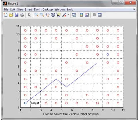
The second simulation result of collision free path for mobile robot is demonstrated in Figure 9. In this simulation plot, there are forty-one obstacles are positioned on the map by random position. The mobile robot is originated the target by using A star (A*) search algorithm to free the obstacles. The way to arrive at the target is the shortest path and minimum flow path for mobile robot navigation.

Figure 9. Screenshot Result for Second Simulation.

The third simulation result of collision free path for mobile robot is confirmed in Figure 10. In this simulation conspire, there are forty-seven obstacles are situated on the diagram by random position. The mobile robot is instigated the target by using A star (A*) search algorithm to gratis the obstacles. The way to disembark at the target is the shortest path and minimum flow path for mobile robot navigation.

Figure 10. Screenshot Result for Third Simulation.

The fourth simulation result of collision free path for

mobile robot is established in Figure 11. In this simulation scheme, there are sixty-seven obstacles are located on the illustration by random position. The mobile robot is initiated the target by using A star (A*) search algorithm to free the obstacles. The way to go ashore at the target is the shortest path and minimum flow path for mobile robot navigation.

Figure 11. Screenshot Result for Fourth Simulation.

The fifth simulation result of collision free path for mobile robot is recognized in Figure 12. In this simulation design, there are fifty-nine obstacles are sited on the figure by random position. The mobile robot is started the target by using A star (A*) search algorithm to free the obstacles. The way to land at the target is the shortest path and minimum flow path for mobile robot navigation.

Figure 12. Screenshot Result for Fifth Simulation.

(8)

obstacles around the target by closed terrain rules. Therefore the mobile robot cannot be reached at that target node normally.

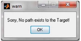
At this time, the warning window for no path exists to the target is displayed and the mobile robot cannot move to get to the specified target node. The information of warning window is shown in Figure 13.

Figure 13. Screenshot Result for Collision Free Path with Closed Terrain.

Figure 14. Warning Window for No Path Exist to the Target.

6. Conclusion

A* path-finding search algorithm is very famous in games for finding shortest distance between two nodes. Today’s games have thousands of agents moving at a same time in the presence of obstacles. Thus it has become very important to find shortest paths concurrently and in a speedy way. Making use of Mobile robot system nature suits this scenario perfectly. Implementing Simple A* algorithm using arrays (Parallel A*) has approximately the same results as compared to A* implementation using adjacent lists. Both implementations are greedy for space. Increase in the size of map increases the memory requirements and thus decreases the speed of algorithm. To further increase the overall performance of algorithm, the memory requirements must be reduced. One option is to use the fast, read-only constant memory for storing the map. Pre-computing some paths and then sharing this already computed information with other agents further increases the efficiency. Another solution to this problem is to exploit the parallel hardware architecture in a true sense. Some improvements are made in the basic A* algorithm to calculate each path using multiple threads that run concurrently and use

shared memory and thread synchronization. It reduces the total search time of A* algorithm as compared to the Parallel A* implementation.

References

[1] RAFIA INAM, “A* Algorithm for Multicore Graphics Processors”, Department of Computer Science and Engineering Division of Computer Engineering, CHALMERS UNIVERSITY OF TECHNOLOGY, 2009.

[2] P.E. Hart, N.J.Nilsson, and B. Raphael, "A formal basis for the heuristic determination of minimum cost paths". IEEE Transactions on System Science and Cybemetics. 4 pp 100-107, 1968.

[3] Rina Dechter and Judea Pearl, “Generalized best-first search strategies and the optimality of A*”, Journal of The ACM, Volume 32, Issue 3, Pages: 505 - 536, 1985.

[4] R. E. Korf, “Depth First Iterative Deeping: An Optimal Admissible Tree Search”, Journal of Artificial Intelligence, pp. 97-100, 1985.

[5] R. E. Korf, “Real-time Heuristic Search”. Artificial Intelligence, 42(2- 3), pp. 189-211, 1990.

[6] R. Holte, M. Perez, R. Zimmer, and A. MacDonald. “Hierarchical A*: Searching Abstraction Hierarchies Efficiently”. In Proceedings AAAI-96, pp. 530-535, 1996. [7] R. Holte, T. Mkadmi, R. Zimmer, and A. MacDonald.

“Speeding Up Problem-Solving by Abstraction: A Graph Oriented Approach”. Artificial Intelligence Journal, 85(1-2), pp. 321-361, 1996.

[8] Samuel Grant Dawson Williams, “Using the A-Star Path-Finding Algorithm for Solving General and Constrained Inverse Kinematics Problems”, Japan, 2008.

[9] Mohd Azlan Shah Abd Rahim and Illani Mohd Nawi, “Path Planning Automated Guided Robot”, Proceedings of the World Congress on Engineering and Computer Science 2008 WCECS 2008, October 22 - 24, 2008, San Francisco, USA, 2008. [10] Bruno Siciliano, Lorenzo Sciavicco, Luigi Villani, and

Giuseppe Oriolo, “Robotics Modelling, Planning and Control”, Spain, 2009.

[11] Giacomo Nannicini, “Point-to-Point Shortest Paths on Dynamic Time-Dependent Road Networks”, French, 2009. [12] Rehman Tariq Butt, “Performance Comparison of AI

Algorithms Anytime Algorithms”, Sweden, 2008.

[13] Muntasir Raihan Rahman, “On-Line Algorithms for Rankings of Graphs”, Bangladesh, 2006.

[14] Subramanian MB, Sudhagar K, Rajarajeswari G. Design of navigation control architecture for an autonomous mobile robot agent. Indian Journal of Science and Technology. 2016 Mar; 9(10). Doi no: 10.17485/ijst/2016/v9i10/85769.

(9)

[16] Murikipudi A, Prakash V, Vigneswaran T. Performance analysis of real time operating system with general purpose operating system for mobile robotic system. Indian Journal of Science and Technology. 2015 Aug; 8(18). Doi no:10.17485/ijst/2015/v8i19/77017.