Load Flow Analysis Using MI Power Software

(1)

IJSRR, 8(2) April. – June., 2019 Page 75

Research article Available online www.ijsrr.org

ISSN: 2279–0543

International Journal of Scientific Research and Reviews

Load Flow Analysis Using MI Power Softwa

Sweta Shah

1

and Sumit Gupta

2*

Indus University Ahmedabad Indus University Ahmedabad Student (M-TECH EPS) Email:Swetashah.el@indusuni.ac.in1, guptasumit8831@gmail.com2*

ABSTRACT

The paper helps to know the basic of Optimal Load Flow Analysis of power system. Load

Flow Analysis are used to validate that the power transfer from generators to consumers through the

grid system is stable, reliable and economical. Load flow analysis is very useful for stabilityanalysis,

future expansion planning and in determining the best economical operation for existing systems.

Load flow analysis also helpful for now the proper setting of the protection devices. Power system

analysis also help to ensure to know that the safe operation of cables, transformer, transmission lines

and other components of power system. Various data of power system like active power, reactive

power,load

angle,

power

factor,

thermal

limit

are

has

to

be

known.

KEYWORDS

: Load flow analysis, contingency analysis, line loading, power system operation.

*Corresponding author:

Sumit Gupta

Indus University Ahmedabad Indus University

Ahmedabad Student (M-TECH EPS)

(2)

1.INTRDUCTION

A well-designed system saves on cost in implementing and maintenance. The primary tools

for analysis for steady state operation is so called power flow analysis or Load flow studies where

the voltage and power flow through the system is determined

1

. Another very popular steady state

analysis tool is the short circuit analysis for determining the fault current through system. Load flow

analysis helps us to determine flows of power in system during normal and emergency conditions

and study the transient behaviour of the system resulting from fault conditions and switching

operations.

A power system is "secure" when it can withstand the loss of one or more elements and

still continue operation without major problems.

OBJECTIVES OF POWER SYSTEM STUDY



Power flow analysis is very important in planning stages of new networks or addition to

existing ones like adding new generator sites, meeting increase load demand and locating

new transmission sites.



It is helpful in determining the best location as well as optimal capacity of proposed

generating station, substation and new lines.



The line status should be known. The line should be not overvoltage it means it should not

operate near the thermal limit or closed to stability.

2. LOAD FLOW ANALYSIS

Power flow analysis is the backbone of power system analysis and design.

The most

important information is known from the load flow is the voltage profile in the system If voltage

variesin the system, large reactive power due to which there is increase in real power loss and in

some extreme cases voltage collapse

2

.If due to demand increase additional lines is to be required a

load flow analysis is help how it will relieve overload adjacent lines. With the help of load flow

analysis one can also know the study performance of the Transformer, Transmission line, and

Generator at steady state

3

. For load flow analysis there are various methods like N-R METHOD,

GAUSS-SIEDEL METHOD, FAST ECOUPLE LOAD FLOW METHOD, among this we are using

the N-R METHOD which has the below benefits among the other methods.

LOAD FLOW TECHNIQUES

(3)

Advantages of N-R METHOD



One of the fastest method convergences to the root



Easy to convert to multiple dimensions



More accurate and not sensitive to the factors such like slack bus selection, regulation

transformers etc. and the number of iterations required in this method is almost independent

of system size

Figure:1 Load flow studies method

3. MI POWER SOFTWARE

(4)

4.SYSTEM UNDER SYUDY

Figure:2 shows the single line diagram of the system under study in MI Power software.

Table:1 Load Details

LOAD DETAILS

BUS NO MW MVAR

BUS 2 21.7 12.7

BUS 3 94.2 19.00

BUS 4 47.8 3.9

BUS 5 7.6 1.6

BUS 6 11.2 7.5

BUS 9 29.5 16.6

BUS 10 9.0 5.8

BUS 11 3.5 1.8

BUS 12 6.1 1.6

BUS 13 13.5 5.8

(5)

Table: 2 components details

Table: 3 Bus voltage details

The effective and most reliable amongst the three load flow methods is the Newton-Raphson method because

it converges fast and is more accurate. In the load flow analysis methods simulated, the tolerance values used

for simulation are 0.001 and 0.1.

5. RESULT FILE

Table: 4 BUS VOLTAGE AND POWER WITHOUT ANY CONTIGENCY Numbers of components

Sr no DESCRIPTION No

1 Bus Number Used 14

2 Transmission Lines 20

3 Generator 3

4 Loads 12

BUS NO. KV BUS NO. KV

1 220 10 220

2 220 11 220

3 220 12 220

4 220 13 220

5 220 14 220

6 220

7 220

8 220

9 220

BUS VOLTAGE AND POWER WITHOUT ANY CONTIGENCY

Bus

No.

Bus Voltage

Generation

Load

Magnitude

Phase Angle

Real

Reactive

Real

Reactive

Per Unit

Degrees

MW

MVAR

MW

MVAR

1 1 0 303.126 200.285 0 0

2 0.6338 -915.24 40 977.19 28.544 16.705

3 0.1027 228.51 0 22.826 9.549 1.926

4 -0.0256 -3309.17 0 0 2.539 -0.207

5 -0.0011 -311.55 0 0 -0.12 -0.025

6 -0.0125 -1388.17 0 0 -0.241 0.161

7 -0.0029 -1280.25 0 0 0 0

8 -0.0029 -1280.25 0 0 0 0

9 -0.0584 -1735.4 0 0 -3.136 1.765

10 0 -1823.22 0 0 0 0

11 -0.0062 163.31 0 0 -0.029 -0.015

12 0.0019 -869.6 0 0 0.006 0.002

13 0.0002 -1794.86 0 0 -0.006 -0.003

(6)

Table: 5 BUS VOLTAGE AND POWER WITH CONTIGENCY WHEN GENERATOR 1 IS OPEN

Table: 6 BUS VOLTAGE AND POWER WITH ANY CONTIGENCY WHEN LINE 1-2 OPEN

BUS VOLTAGE AND POWER WITH CONTIGENCY WHEN GENERATOR 1 IS OPEN

Bus

No.

Bus Voltage

Generation

Load

Magnitude

Phase Angle

Real

Reactive

Real

Reactive

Per Unit

Degrees

MW

MVAR

MW

MVAR

1 0.8052 -2.48 0 0 0 0

2 1 0 278.444 262.546 21.7 12.7

3 0.5977 -26.28 0 24.94 89.573 18.067

4 0.518 -17.73 0 0 41.539 3.389

5 0.6129 -6.47 0 0 7.023 1.478

6 0.1754 -14.55 0 0 3.659 2.45

7 0.3714 -21.1 0 0 0 0

8 0.3714 -21.1 0 0 0 0

9 0.2246 -25.88 0 0 15.21 8.559

10 0.1794 -22.39 0 0 4.393 2.831

11 0.17 -22.73 0 0 1.44 0.741

12 0 -64.88 0 0 0 0

13 -0.0001 -55.18 0 0 -0.002 -0.001

14 0 -70.41 0 0 0.002 0.001

BUS VOLTAGE AND POWER WITH ANY CONTIGENCY WHEN LINE 1-2 OPEN

Bus

No.

Bus Voltage

Generation

Load

Magnitude

Phase Angle

Real

Reactive

Real

Reactive

Per Unit

Degrees

MW

MVAR

MW

MVAR

1 1 0 114.073 234.035 0 0

2 2.902 107138.6 40 340.47 55.812 32.664

3 3.0994 105526.6 0 3098.696 2385.045 481.06

4 2.7022 133386.8 0 0 11.454 0.935

5 1.0354 45045.91 0 0 -0.1 -0.021

6 -1.233 129871.3 0 0 9.799 6.562

7 -3.9145 6415.1 0 0 0 0

8 -0.9141 6145.11 0 0 0 0

9 0.6095 12059.45 0 0 29.5 16.6

10 3.2485 716.46 0 0 9 5.8

11 0.5582 -5308.6 0 0 3.5 1.8

12 1.1745 130531.4 0 0 1.439 0.377

13 -0.0165 24671 0 0 -0.254 -0.109

(7)

Table: 7 LINE FLOW AND LINE LOSSES WITH CONTIGENCY LINE1-2 OPEN

LINE FLOW AND LINE LOSSES WITH CONTIGENCY LINE1-2 OPEN

SR No.

FORWARD Loss

FROM

NODE TO NODE

Real Reactive Real Reactive

MW MVAR MW MVAR

1 BUS 1 BUS 2 LINE IS OPEN

2 BUS 2 BUS 3 2260.177 3869.126 4075.205 8297.273

3 BUS 2 BUS 4 1154.827 -63.267 271.4895 552.763

4 BUS 1 BUS 5 -140.365 149.284 71.7703 146.1271

5 BUS 2 BUS 5 1385.428 2595.702 1757.069 3577.459

6 BUS 3 BUS 4 584.258 4323.327 3386.545 6895.136

7 BUS 4 BUS 5 1485.64 1992.248 1445.766 2943.635

8 BUS 5 BUS 6 -190.502 144.128 90.9881 185.2552

9 BUS 4 BUS 7 -1080.48 -256.872 288.7302 587.8657

10 BUS 7 BUS 8 -0.253 0.58 0 0.001

11 BUS 4 BUS 9 396.3 1288.293 501.0.334 1020.123

12 BUS7 BUS 9 1736.786 2931.942 1295.407 2637.497

13 BUS 9 BUS 10 243.186 555.429 1691.728 3444.422

14 BUS 6 BUS 11 94.406 192.715 51.7759 105.4177

15 BUS 6 BUS 12 -34.588 662.56 494.8986 1007.632

16 BUS 6 BUS 13 177.199 348.873 172.1127 350.428

17 BUS 9 BUS 14 54.367 94.995 55.126 112.2386

18 BUS 10 BUS 11 799.417 2684.56 1270.823 2587.444

19 BUS12 BUS 13 157.355 324.346 161.0.222 327.8473

(8)

IJSRR, 8(2) April. – June., 2019 Page 82 Table: 8LINE FLOW AND LINE LOSSES WITHOUT CONTIGENCY

LINE FLOW AND LINE LOSSES WITHOUT CONTIGENCY

SR No.

FORWARD Loss

FROM NODE TO NODE Real Reactive Real Reactive

1 BUS 1 BUS 2 82.744 70.98 20.3143 41.3608

2 BUS 2 BUS 3 62.463 93.03 53.4213 108.7677

3 BUS 2 BUS 4 43.728 96.711 47.9284 97.5841

4 BUS 1 BUS 5 113.966 231.57 113.8615 231.8264

5 BUS 2 BUS 5 45.855 93.005 45.7479 93.1455

6 BUS 3 BUS 4 1.877 2.458 1.5509 3.1577

7 BUS 4 BUS 5 0.07 0.158 0.0777 0.1581

8 BUS 5 BUS 6 -0.002 -0.003 0.0148 0.0302

9 BUS 4 BUS 7 0.093 0.157 0.0867 0.1765

10 BUS 7 BUS 8 0 0 0 0

11 BUS 4 BUS 9 -0.058 0.515 0.6985 1.4221

12 BUS7 BUS 9 0.042 -0.014 0.3927 0.7906

13 BUS 9 BUS 10 0.388 0.791 0.3883 0.7906

14 BUS 6 BUS 11 0.004 0.051 0.0287 0.0584

15 BUS 6 BUS 12 0.017 0.03 0.013 0.0266

16 BUS 6 BUS 13 0.018 0.037 0.0181 0.0369

17 BUS 9 BUS 14 0.52 0.771 0.4333 0.8822

18 BUS 10 BUS 11 0 0 0.0044 0.009

19 BUS12 BUS 13 0 0.001 0.0005 0.001

(9)

IJSRR, 8(2) April. – June., 2019 Page 83 Table: 9 LINE FLOW AND LINE LOSSES WIH CONTIGENCY GENERATOR 1

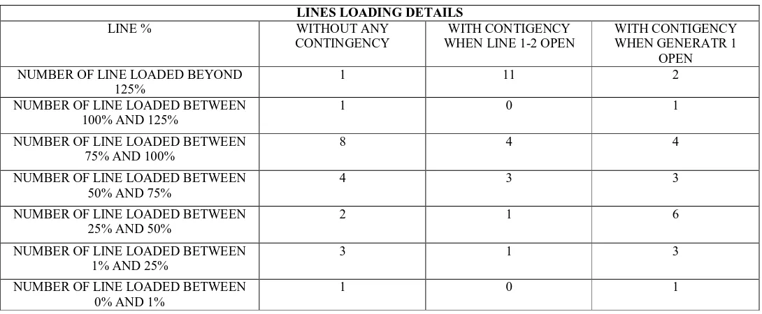
Table :10 LINES LOADING DETAILS

LINE FLOW AND LINE LOSSES WITH CONTIGENCY GENERATOR 1

SR No.

FORWARD Loss

FROM NODE TO NODE Real Reactive Real Reactive

1 BUS 1 BUS 2 -25.06 -32.172 4.484 9.1296

2 BUS 2 BUS 3 114.022 77.331 32.444 66.058

3 BUS 2 BUS 4 94.127 99.348 32.015 65.1837

4 BUS 1 BUS 5 25.709 32.232 4.481 9.1235

5 BUS 2 BUS 5 60.456 82.672 17.9299 36.506

6 BUS 3 BUS 4 -4.837 17.066 1.5052 3.0646

7 BUS 4 BUS 5 -19.243 -2.915 2.4132 4.9134

8 BUS 5 BUS 6 34.099 60.587 21.9971 44.877

9 BUS 4 BUS 7 11.284 16.362 2.5169 5.1244

10 BUS 7 BUS 8 0 0 0 0

11 BUS 4 BUS 9 21.23 33.58 10.0559 20.4742

12 BUS7 BUS 9 7.846 11.907 2.5196 5.129

13 BUS 9 BUS 10 0.591 2.641 0.2484 0.5057

14 BUS 6 BUS 11 1.125 -0.191 0.0723 0.1473

15 BUS 6 BUS 12 3.499 7.125 3.4994 7.1249

16 BUS 6 BUS 13 3.499 7.128 3.5014 7.129

17 BUS 9 BUS 14 5.734 11.67 5.7314 11.6695

18 BUS 10 BUS 11 0.236 0.373 0.0103 0.021

19 BUS12 BUS 13 0 0 0 0

20 BUS 13 BUS 14 0 0 0 0

LINES LOADING DETAILS

LINE % WITHOUT ANY

CONTINGENCY

WITH CONTIGENCY WHEN LINE 1-2 OPEN

WITH CONTIGENCY WHEN GENERATR 1

OPEN NUMBER OF LINE LOADED BEYOND

125%

1 11 2

NUMBER OF LINE LOADED BETWEEN 100% AND 125%

1 0 1

8 4 4

4 3 3

2 1 6

3 1 3

(10)