Development and evaluation of a protocol to identify individuals of Trichosurus vulpecula with non-invasively recovered DNA

(1)

Lincoln University Digital Thesis

Copyright

Statement

The

digital

copy

of

this

thesis

is

protected

by

the

Copyright

Act

1994

(New

Zealand).

This

thesis

may

be

consulted

by

you,

provided

you

comply

with

the

provisions

of

the

Act

and

the

following

conditions

of

use:



you

will

use

the

copy

only

for

the

purposes

of

research

or

private

study



_you

_will

_recognise

_the

_author's

_right

_to

_be

_identified

_as

_the

_author

_of

_the

_thesis

_and

due

acknowledgement

will

be

made

to

the

author

where

appropriate



_you

_will

_obtain

_the

_author's

_permission

_before

_publishing

_any

_material

_from

_the

thesis.

(2)

Development and evaluation

of a protocol to identify

individuals of

Trichosurus

vulpecula

with non-invasively

recovered DNA

A thesis

submitted in partial fulfilment of the requirements for the Degree of

Master of Applied Science at

Lincoln University

by

Juan F. Due˜nas-Serrano

(3)

(4)

iii

a mis hermanos: Francisco, Nicol´as y Pamela.

(5)

(6)

Abstract of a thesis submitted in partial fulfilment of the

requirements for the Degree of M.Appl.Sc.

Development and evaluation of a protocol to

identify individuals of

Trichosurus vulpecula

with

non-invasively recovered DNA

by

Juan F. Due˜nas-Serrano

The Australian brushtail possum (Trichosurus vulpecula) is a pervasive

marsupial pest of New Zealand. Impacting on the native flora and fauna

and the nation’s livestock industry by its vectoring of bovine turberculosis,

T. vulpecula is a priority for control and eventual eradication. Current pest

control initiatives involve aerial deployment of chemical poisons, baiting

and trapping. To establish the success of such control operations, estimates

of possum population size pre- and post culling are required. Currently

several monitoring methodologies — requiring the detection and trapping

of individuals — are available to estimate indices of abundance (e.g. the

residual trap-catch index). But these monitoring protocols are constrained

by logistical and analytical considerations. The necessity to overcome the

limitations of traditional monitoring schemes presents the opportunity to

develop and evaluate the implementation of non-invasive genetic monitoring

systems for possums. This thesis aimed to optimise an efficient amplification

system for a panel of eight microsatellite loci that allow the identification of

(7)

vi

a range of conditions, and evaluate the use of salivary DNA retrieved from

interference devices as template for amplification.

Optimisation of amplification conditions for all loci in the panel was

evaluated with DNA extracted from possum tissue collected at three

local-ities in Canterbury region. Allele polymorphism was analysed by capillary

electrophoresis and fluorescence based detection of fragments. After

opti-misation, locus Tv16 was discarded from the panel due to its linkage with

locus Tv27 and amplification of unspecific fragments. Microsatellite

diver-sity patterns of the seven remaining loci revealed moderate to high

poly-morphism and heterozygosity, no evidence of genetic structuring between

localities across Canterbury (Fst = 0.03), and a sufficiently low overall

probability of identity adjusted for siblings (P Isib) (3 ×10−3) to ensure a

robust identification of individual possums based on their multi-locus

geno-type. Further exclusion of locus Tv54 was recommended based on its high

P Isib(0.63–1.00) and incidence of genotyping error.

Amplification of template DNA extracted from tissue was not exempt

from genotyping error (mean error rate per locus (el) = 4,8% and observed

error rate per multi-locus genotype (eobs) = 33.3%), these errors being

as-sociated in equal measure with stochastic causes (e.g. allele drop-out and

false alleles) and systematic causes (e.g. scoring errors, sample swapping or

contamination). No evidence of null alleles was detected.

Six loci were successfully assembled into a multiplex PCR assay. The

implementation of mutliplex PCR had no significant effects on the incidence

of genotyping error or the consistency of allele size estimation compared

to standard PCR, and represented a substantial reduction in labour and

resources needed to obtain a genotype (92% cost reduction relative to

(8)

vii

While 1:6 dilution of DNA extracted from tissue did not show significant

effects on the amplification success and the mean genotyping error rate per

locus, the use of template DNA retrieved from saliva decreased the

perfor-mance of the microsatellite amplification system significantly. Only 18 of 24

samples were able to generate positive or partially positive genotypes, loci

with amplicons>200 bp being the most affected, while the mean error rate

per locus increased to 45%

Altogether, these results indicate that locus characteristics (i.e. amplicon

size) and quality of template DNA are crucial factors affecting the

sensitiv-ity and reliabilsensitiv-ity of the protocol developed. Potential ways to improve the

remote collection of DNA from saliva are recommended.

Keywords: Trichosurus vulpecula, microsatellite markers, probability

of identity, multiplex PCR, amplification success, genotyping error, saliva,

(9)

Acknowledgements

I would like to express my sentiments of gratitude to numerous colleagues,

institutions and friends for supporting me throughout the duration of this

work.

First, I would like to thank my supervisory team of Dr. Rob Cruickshank

and Dr. James Ross for their guidance, disposition and input during the

de-velopment and final accomplishment of this work. Rob patiently introduced

me to the fascinating world of DNA, offering advice on molecular techniques

and giving me much appreciated freedom to venture into the depths of the

molecular ecology laboratory at Lincoln University. James provided

invalu-able assistance with statistical analyses and his ideas enriched the design of

the study. Dr. Hayley Ridgeway assessed the proposal and provided

sug-gestions that greatly improved the study design. Dr. Adrian Paterson read

and commented on early drafts of this thesis and provided relevant

sugges-tions to improve my writing skills. I am especially grateful to Dr. Marie

Hale (Canterbury University, New Zealand), who generously shared the

se-crets of microsatellite data analysis and donated her time for an informative

induction to the mechanics of capillary electrophoresis.

This study would not be possible without the generous collaboration of

the Centre for Wildlife Management and Conservation staff, who helped me

with data collection at the various stages of this study. My gratitude goes to

(10)

ix

Brent Barrett, Matt Kavermann, Shona Sam, Lee Shapiro and Tim Sj¨oberg.

I am also deeply grateful to Mr. Tim Kelly, who assisted with the collection

of tissue samples at Lewis Pass. I wish to also thanks my colleagues at

the molecular ecology laboratory; in particular Jagoba, Emily and Ben, for

sharing their expertise and advice when needed. I am especially indebted to

Norma Merric, who operates the sequencer at the Bio-Protection Research

Center, for selflessly sharing her ample experience in fragment analysis; and

to Candice Barclay, for serving as the bridge between the bio-technology

industry and me.

Several colleagues provided generous assistance with data analysis and

presentation of results. Sam Brown and Ruppert Collins inspired me to try

LA_{TEX and offered advice on how to operate it. Ferran Palero (Institute}

of Science and Technology, Austria) provided feedback for the operation of

MICROSATELIGHT. Dr. Paul Johnson (University of Glasgow, United

Kingdom) offered timely suggestions for the quantification and analysis of

genotyping error. Dr. Paul Moran (NOAA fisheries service, USA) granted

permission for the reproduction of figure 3.1. I would like to express my

debt of gratitude to all the programmers that share the philosophy of open

software.

I gratefully acknowledge the financial assistance the Faculty of

Agricul-ture and Life Sciences at Lincoln University and the Animal Health Board,

through a research grant awarded to Dr. James Ross. I also wish to

ex-tend my debt of gratitude to the people at New Zealand Aid, in particular

Angela Williams and Mandy Buller, for offering me the financial support

to complete my degree in New Zealand, and for timely processing all my

requests.

(11)

x

to pursue my goals, and for offering me their unlimited love in return. To

my friends, for sharing unforgettable adventures through land and sea, and

for providing the necessary humour to bear with the odds of life. I hope

I can repay in some way the time I have been away from you. Finally, to

my dearest Annabel, my partner and love, for all the happiness you bring

to my life, for providing the inspiration to continue against all odds and for

(12)

List of Figures

2.1 Geographic origin of samples collected for this study. BP =

Banks Peninsula, Ho = Hororata and LP = Lewis Pass. . . . 17

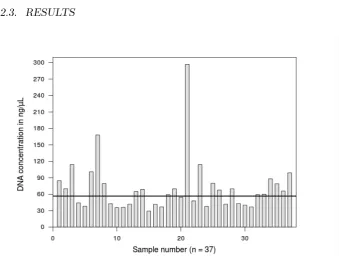
2.2 DNA concentration measured in ng/µL. Bars represent tissue

samples from which DNA was extracted between June-July, 2011. The horizontal line represents the median DNA

con-centration (59.85 ng/µL) . . . 29

2.3 Number of alleles observed across loci and location in

Can-terbury. Numbers on the x-axis represent the different loci in ascending order as follows: 1= Tv19, 2 = Tv27, 3 = Tv53, 4

= Tv54, 5 = Tv58, 6 = Tv5.64 and 7 = TvM1 . . . 30

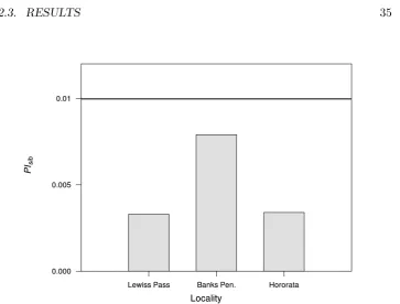
2.4 Probability of identity adjusted for siblings variation across

localities in Canterbury. The horizontal line marks the

mini-mum value of P Isib required to avoid bias in genetic

estima-tors of population size as suggested by Waits et al. (2001)

. . . 35

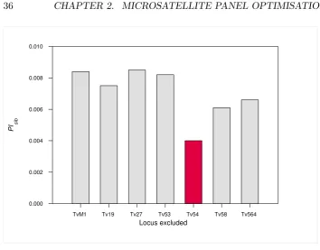
2.5 Contribution of each locus to the magnitude of P Isib. Bars

represent the magnitude of P Isib estimated when the

infor-mation of the locus nominating the bar is missing. The bar

highlighted in red shows the estimatedP Isibwhen locus Tv54

is excluded from the calculations. . . 36

3.1 Illustration of a size shift published in Moran et al. (2006).

The black peaks in the figure represent the same allele but the profiles were obtained with capillary electrophoresis run on different machines. The grey peaks represent the size stan-dard. This figure is reproduced with permission of the author

(Moran, pers. comm. 2012) . . . 47

3.2 MULTIPLEX MANAGER optimal primer set combination.

Boxes represent each of the six loci included in the multiplex assay. The scale on top of the figure is in base pairs and the axis on the left displays the suggested annealing temperature

for PCR . . . 55

(15)

xiv LIST OF FIGURES

3.3 Profile of individual 3 as visualised in Peak Scanner v1.0. The

scale on top of the graph is in base pairs and the x-axis is in relative fluorescent units. A legend with the estimated allele

size is shown below each peak . . . 56

3.4 Linear regression models of allele sizes estimates of products

generated by singleplex and multiplex PCR approaches versus

discrete allele categories designated in chapter 3 . . . 58

3.5 Projection of the cost of genotyping with different

amplifica-tion approaches . . . 61

4.1 Decrease in amplification success due to the interaction

be-tween amplicon size and quantity and quality of template DNA used to generate profiles for individual possums. Letter ‘b’ indicates significant differences between means according

to Fisher’s LSD test (α= 0.05) . . . 77

4.2 Increase in mean error rate per locus according to the

quan-tity and quality of template DNA used to generate profiles of individual possums. Letter ‘b’ indicates significant differences

(16)

List of Tables

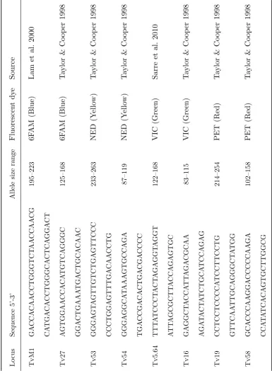
2.1 Characteristics of the 8 loci selected to genotype possums . . 21

2.2 Optimised PCR conditions for sevenamicrosatellite loci . . . . 23

2.3 Number of alleles (A), number of private alleles (PA),

ob-served (Ho) and expected (He) heterozygosity and inbreeding

coefficient (Fis) for every locus by location sampled in

Can-terbury. Population structure coefficient (Fst) estimated for

each locus in Canterbury . . . 32

2.4 Summary of statistical parameters estimated per locus at each

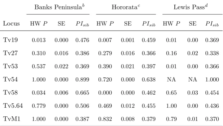
of the localities sampled in Canterbury. The Hardy-Weinberg

(HW) exact probability test P-values (HW P)a and their

standard error (SE) as well as the P Isib for every locus are

presented in this table . . . 33

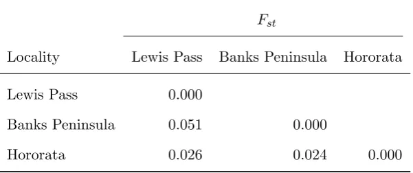
2.5 Pairwise comparison matrix of genetic structure (Fst)

be-tween localities sampled in Canterbury . . . 34

3.1 Summary of linear regression parameters between

amplifica-tion approaches. P-values correspond to ANCOVA’s results

of treatment effects. A non-significant result suggests there is no significant difference between the intercept values - i.e.

there is no treatment effect . . . 59

3.2 Summary of genotyping error categories found by comparing

singleplex replicates with multiplex replicates . . . 60

3.3 PCR costs (NZD) per sample unit as incurred by different

amplification approaches . . . 61

4.1 Summary of amplification success (success), per locus allele

drop-out rate (per locus allele drop-out rate (pl)) and per

locus false allele rate (per locus false allele rate (fl)) for

repli-cates obtained from diluted DNA template. Only error rate

per locus (el) is presented for replicates obtained from

Wax-Tags (Waxtags) . . . 76

(17)

Abbreviations

NIGM non-invasive genetic monitoring

SSR short sequence repeats

NPCA National Possum Control Agency

RTCI residual trap catch-index

CWMC Centre for Wildlife Management and Conservation

MHC major histocompatibility complex

HW Hardy-Weinberg

ANOVA analysis of variance

CO-I barcoding region of the mitochondrial cytochrome oxydase sub-unit

I gene

ANCOVA analysis of covariance

(18)

Chapter 1

Introduction

1.1 Non-invasive genetic monitoring

In the past decade molecular ecology has become established as an important

sub-discipline of ecology (Rieseberg et al., 2010). Molecular ecology applies

popular molecular biology techniques, such as the polymerase chain reaction

(PCR) or DNA sequencing, to quantify the genetic diversity of organisms,

populations and communities while answering questions about their ecology

(Freeland et al., 2011; Beebee & Rowe, 2008). The link between genetic

diversity and ecology provides new insights to topics that have been

tra-ditionally addressed with field techniques, such as population demography

(Banks et al., 2003), host-parasite (Luikart et al., 2008a) or predator-prey

interactions (Blejwas et al., 2006), to name a few. An increasing number

of reviews across several sub-disciplines of ecology examine the potential of

molecular approaches to further enrich their varied list of methodological

strategies (Waits & Paetkau, 2005; Sarre & Georges, 2009; Schwartz et al.,

2007). In many situations the creative use of molecular ecology approaches

can infer answers to questions that would be impractical to address using

(19)

2 CHAPTER 1. INTRODUCTION

traditional techniques (e.g. the inference of historical population expansion,

Curtis et al., 2009). The identification of individuals within a population

— in order to determine the census population size — is one of the most

widely studied applications of molecular ecology and constitutes the focus

of this work.

Census population size (Nc) is defined as the number of individuals

con-stituting a population at any given point in time (used synonymously with

abundance in some texts, Freeland et al., 2011; Morrison, 2009; Mills, 2007).

Scientists estimatingNcmust be able to reliably detect and identify

individ-uals of the targeted species. This can involve conducting surveys that

tar-get and count individuals, made difficult and expensive if the species under

study is elusive or distributed over a large area. Data generated from such

surveys can be analysed with rarefaction curves, capture-mark-recapture

ex-periments or occupancy models to gain an estimate of Nc (Borchers et al.,

2002; Sinclair, 2006; MacKenzie et al., 2006). A complication to the

esti-mation ofNcarises because the concept of population has many definitions

(Morrison, 2009), and surveys can only cover limited geographic regions.

To overcome some of the logistical and conceptual issues of estimating

Nc, a set of alternative parameters known as indices of abundance have been

defined (Williams et al., 2002). For example, density is an index that counts

the number of individuals per unit of area. One assumption of indices of

abundance is that all individuals in the population have constant detection

probabilities (Mills, 2007), but if this is false, the relationship between

in-dices of abundance andNc is obscured. Despite this limitation, a moderate

level of imprecision of population size estimates is tolerated more easily than

the impracticalities of measuring Nc with the result that wildlife

(20)

1.1. NON-INVASIVE GENETIC MONITORING 3

(Warburton, 2000).

Further alternatives to traditional surveying methods and indices of

abundance lie in the developing field of non-invasive genetic monitoring

(NIGM). NIGM, as the name suggests, involves non-invasively collecting

samples such as hair or faeces from which DNA can be retrieved. NIGM

uses molecular markers, such as microsatellites or single nucleotide

polymor-phisms (SNP’s), to generate a genotype, or fingerprint, of each individual

within a population using the DNA collected. Unique genotypes can be

later used to estimate ˆNc using similar analytical approaches to those used

for traditional monitoring techniques. For instance, when using genetic data

for mark-capture-recapture analysis, a genotype can be considered a capture

while a repeated detection of the same genotype is considered a recapture

(for a detailed review ofNcestimation using genetic data see Luikart et al.,

2010).

NIGM possesses two important characteristics that make it an

attrac-tive monitoring scheme for wildlife management: universality and

versatil-ity. Universality because virtually all living organisms can be detected or

monitored by retrieving their DNA. Versatility because over the last decade

progress in this field has made it possible to generate reliable genotypes from

minute amounts of template DNA - as little as 1 ng or less (Benschop et al.,

2011; Petricevic et al., 2010). With the reduced amount of template DNA

required, the number of sources that DNA can be obtained from is

virtu-ally endless. Hair follicles and intestinal cells present on fresh faeces of free

ranging animals are currently the most commonly used samples for wildlife

management applications (Broquet et al., 2007b). These achievements have

been made possible by a suite of technical improvements primarily

(21)

The unique characteristics of NIGM have sparked an interest in

evaluat-ing this approach for an increasevaluat-ing range of non-model organisms and under

a variety of contexts. While traditionally data from NIGM has been

ap-plied to species and individual identification, kinship analysis, dispersal and

estimation of population size (DeYoung & Honeycutt, 2005; Luikart et al.,

2010); the information generated by this method is also suitable for the

study of population genetics and short-term evolution of species (Hamilton,

2009; Palstra & Ruzzante, 2008). For instance, information gathered during

NIGM regimes can help in the interpretation of the mechanisms of

establish-ment and spread of founding populations, or to determine if hybridisation

counters the deleterious effects of inbreeding or loss of evolutionary

poten-tial (Allendorf & Luikart, 2007). Assessment of populations to gain such

information is a critical first step in devising management plans of invasive

species making NIGM increasingly important in effective monitoring efforts.

1.2 NIGM and Pest Management in New Zealand

The implementation of advanced monitoring methods for improved

manage-ment of invasive species is of particular importance for New Zealand. One

such species, constituting a significant threat to the country’s indigenous

biota and livestock industry, is the Australian brushtail possum

Trichosu-rus vulpecula. Because of the direct and indirect negative interactions of

T. vulpecula with native flora and fauna and its vectoring of bovine

tu-berculosis, extensive control operations are commonly undertaken in New

Zealand rural areas (O’Reilly-Wapstra & Cowan, 2010; Sweetapple &

Nu-gent, 2009). Control is primarily by means of aerial delivery of sodium

fluoroacetate (1080) or ground-based deployment of toxic baits. Once

(22)

1.2. NIGM AND PEST MANAGEMENT IN NEW ZEALAND 5

in order to prevent future outbreaks, guide subsequent control efforts, and

evaluate the work of private contractors (Warburton, 2000). This requires a

monitoring method that accurately estimates population size pre- and

post-control. It is desirable that the monitoring method also allows additional

information to be collected, such as patterns of aggregation and movement

of surviving individuals (Brown et al., 2004; Cowan et al., 2002; Pech et al.,

2010), or quantification of the re-invasion rate of control areas (Gleeson

et al., 2010). In order to determine these factors, the National Possum

Con-trol Agency (NPCA) currently uses the residual trap catch-index (RTCI)

(National Possum Control Agencies, 2008a; Warburton et al., 2004). The

RTCI is a standardised index of abundance for possums and is relatively

robust. However, RTCI suffers from several logistical and analytical

limita-tions. First, the RTCI protocol requires the deployment of bulky equipment

— leg-hold traps — and subsequent visits to these devices across extensive

areas of often rugged terrain; second, the deployment of devices poses an

unintended risk of interaction with endangered flightless birds such as the

wekaGallirallus australis and kiwi Apteryx spp.; third, a recent study

sug-gested that RTCI estimates have a non-linear relationship with population

size due to seasonal and density dependent variation in detection

probabil-ities (Forsyth et al., 2005). Despite these limitations, equally robust and

more cost effective methods for estimating possum abundance are currently

unavailable for widespread adoption.

A possible alternative for replacement of RTCI as the possum

monitor-ing standard makes use of WaxTags and is under development by the NPCA

(National Possum Control Agencies, 2008b). Waxtags are interference

de-vices consisting of wax blocks attached to visual lures. When compared to

(23)

while the indices of abundance derived from them (i.e. tag station index and

the bite-mark index) are consistent with the RTCI (Thomas et al., 2003;

Ogilvie et al., 2006). Thomas et al. (2007) also concluded that the

bite-mark index robustly reflects changes in possum population size comparable

to RTCI. Yet the accuracy of the bite-mark index has been questioned.

In-dices of abundance derived from Waxtags appear to lose sensitivity in

detect-ing population size changes when possum populations are either extremely

large or small (Morgan et al., 2007; Warburton et al., 2004). A common

ar-gument against the use of abundance indices derived from Waxtags is that

the use of lures to attract possums towards Waxtags triggers a behavioural

response known as contagion. Contagion occurs when an individual actively

seeks and bites several Waxtags on a given sampling occasion, which if

un-noticed can bias the estimate of the bite-mark index (Thomas et al., 2003;

Sargeant et al., 1998; Warburton, 2000).

In an attempt to further develop the Waxtags method, Vargas et al.

(2009) were able to amplify the barcoding region of the mitochondrial

cy-tochrome oxydase sub-unit I gene (CO-I) from DNA found on traces of

saliva collected using Waxtags. Currently, saliva retrieved from Waxtags is

an attractive substrate of remotely-collected possum DNA, given that

pre-liminary studies have established major logistical constraints of obtaining

DNA of this possum species from hair follicles and faecal samples (Gleeson

et al., 2003; Morgan et al., 2007). Saliva presents a challenge and also a

new and promising opportunity to test the ability of Waxtags to aid and

better inform allocation of possum control operations. If Waxtags allow the

retrieval of DNA of sufficient quantity and quality in order to conduct

reli-able genotyping assays, Nc can be directly determined, potentially offering

(24)

1.3. MARKER SELECTION 7

1.3 Marker selection

In order to answer a variety of different ecological questions with genetic

in-formation, marker selection is critical. The progress in molecular biology has

increased the availability of markers to choose from, each with limitations

and therefore suited for a particular use.

Microsatellites are frequently used in studies involving population size

estimation. Microsatellites or short sequence repeats (SSR) are non-coding

regions of DNA conformed by a variable number of tandem repeats of a short

sequence motif, generally of one to six nucleotides (Allendorf & Luikart,

2007). Variation in the number of repeats gives microsatellites the

interest-ing property of havinterest-ing more than one allele, or polymorphism. It is

acknowl-edged that microsatellite polymorphism is the result of a high mutation rate

relative to the rest of the genome (10−2 _{to 10}−6 _{nucleotides per locus, per}

generation,sensu Oliveira et al., 2006). However, the proposed causes (e.g.

polymerase slippage or unequal crossing over) and accompanying

theoreti-cal models explaining the high mutation rate are numerous (Buschiazzo &

Gemmell, 2006, and references therein) and ultimately have profound

impli-cations on the way genetic parameters of population differentiation, such as

Fst (Balloux & Lugon-Moulin, 2002), are estimated.

When it comes to discriminating individuals, a task requiring the use

of highly polymorphic markers to quantify genetic differences at such fine

scales, microsatellite usage is widespread. While there is a variety of similar

polymorphic markers such as allozymes or restriction fragment length

poly-morphism (RFLP’s), microsatellites are generally preferred because of their

co-dominant nature, reproducibility among studies and increased power for

statistical analysis. However, the popularity of microsatellites has been

(25)

which unlike microsatellites have a well defined model of mutation and are

therefore easier to score, do not require calibration when transfering

be-tween laboratories, and are amenable to different forms of typing (Garvin

et al., 2010). Although SNPs have several desirable properties, in some

sit-uations microsatellites can prove a superior choice. Unlike SNPs, primers

of microstellites can be transferred across taxa and errors associated with

genotyping can be identified and tracked (Guichoux et al., 2011a). In the

end, the choice of marker will be governed by reasons of practicality and

economy of application.

Taylor & Cooper (1998) isolated a panel of eight microsatellite loci for

T. vulpecula. This work provided future researchers with tools to study the

genetic structure of both introduced and native populations of this species.

Since then, this panel has been used in studies focused on gaining insights

into the reproductive system of T. vulpecula in their native (Clinchy et al.,

2004) and introduced ranges (Taylor et al., 2000); and understanding the

ge-netic structure and relationships of introduced populations in New Zealand

(Taylor et al., 2004). To date, one attempt has been made (using scats) to

test these microsatellites in the context of NIGM (Morgan et al., 2007). In

2000, Lam et al. reported a microsatellite locus located within an intron of

the major histocompatibility complex (MHC) gene region. This locus has

since been used in combination with some of the microsatellites described by

Taylor & Cooper (1998), in studies that examine the patterns of dispersal of

T. vulpecula remnant populations in urban Australia (Stow et al., 2006) and

to study the relationship of adult survival and genetic diversity of a closely

related speciesTrichosurus cunninghami (Banks et al., 2008). Finally, very

recently Sarre et al. (2010) described another set of microsatellite markers

(26)

1.4. NIGM LIMITATIONS 9

to a more effective control allocation is yet to be fully explored.

1.4 NIGM limitations

Genotyping of DNA collected from non-invasive sources poses a series of

challenges. The first set of complications occur during allele amplification.

Low quantity and quality of DNA collected from sources such as hair or

saliva, may generate a unique kind of stochastic error - genotyping error.

Genotyping error manifests in a variety of ways of which the most commonly

reported are: 1) allele drop-out (i.e. failure to amplify one of the alleles of

an heterozygote individual) and 2) false alleles (the erroneous scoring of

“stuttering” peaks as true alleles) (Taberlet et al., 1996). Regardless of

the type of error, the magnitude of genotyping error can seriously limit the

ability of NIGM to yield accurate population size estimates (see reviews by

Bonin et al., 2004; Broquet & Petit, 2004; DeWoody et al., 2006; Pompanon

et al., 2005). For instance, Waits & Leberg (2000) determined that a per

locus error rate as low as 0.05 can introduce a 200% bias on population

size estimates. Furthermore, failure to quantify and monitor genotyping

error occurrence can confound the conclusions of a broad range of studies.

Hoffman & Amos (2005), in their study of paternity assignment of antartic

fur seals Arctocephalus gazella, determined that error rates as low as 0.13–

0.74% per sample resulted in the incorrect assignment of 4.9% of paternities.

The occurrence of stochastic genotyping error is often associated with the

characteristics of each locus and the level of optimisation of the reaction

con-ditions at which they were processed. For instance, loci that target relatively

large amplicons (>200 bp) may perform poorly with highly degraded DNA

(Broquet et al., 2007b), while poorly optimised reaction conditions may

(27)

and primer dimers (reviewed in Guichoux et al., 2011a). Genotyping error is

also often associated with low quantity and quality of template DNA, which

is a common occurrence in non-invasively collected samples. But there is

uncertainty, as to which of this two characteristics — quantity or quality —

influences the occurrence of genotyping error more significantly. It is clear

by this evidence, that once a panel of markers has been selected it is

criti-cal to optimise the markers individually while quantifying the occurrence of

error in order to detect its causes.

A further complication of the genotyping process lies in errors that may

arise during two distinct processes leading to the scoring of true or

“under-lying” alleles. These processes are known as sizing and binning. Both tasks,

while conceptually simple, may induce the occurrence of human errors that

will eventually have pervasive consequences on the final quality of

genotyp-ing data (Pompanon et al., 2005; Guichoux et al., 2011a). For instance,

Hoffman & Amos (2005) attributed an important percentage of the total

er-rors detected in their study to human erer-rors (57.4%). The specific problems

that allele sizing and binning may cause can be clarified and mitigated by

understanding how these processes operate.

In the case of allele sizing, specialised software detects the presence of

a peak representing a fragment and estimates its length by implementing

a series of complex algorithms. Size-calling algorithms use a size standard

— a collection of DNA fragments of known size all labelled with the same

fluorocrome that is co-injected into the capillary of a sequencer along with

the sample of interest — as a reference to estimate the length of a fragment

(e.g. size-matching algorithm, Applied Biosystems 2005). Despite the sizing

process being perceived as highly reproducible, in recent years a variety of

(28)

1.4. NIGM LIMITATIONS 11

Pasqualotto et al. (2007) reported differences of up to 5 nucleotides between

the size of a fragment determined by sequencing and the size estimated with

capillary electrophoresis. Other studies have reported differences in the size

of alleles scored using different machines (LaHood et al., 2002; Ellis et al.,

2011). Causes for this discrepancies may be varied, but it has been suggested

that nucleotide composition of microsatellite flaking sequences, fluorochrome

dye characteristics, differences in sequencer platforms, migration deviations

of the internal size standard, nature of the gel matrix used and even the

room temperature at the moment of electrophoresis can cause shifts in the

mobility of alleles, therefore producing slightly different size estimates of

the same alleles (Haberl & Tautz, 1999; Pasqualotto et al., 2007; LaHood

et al., 2002; Sutton et al., 2011). Mobility shifts can be a serious problem

that should not be overlooked, particularly when the goal is to standardise

microsatellite typing protocols across laboratories (Pasqualotto et al., 2007;

Moran et al., 2006; Ellis et al., 2011).

Binning raises a different set of issues. Because allele length estimates

are expressed as decimal values, such data needs further processing to

as-sign discrete allele categories. In well studied organisms, such as humans,

this task is performed by comparing allele length estimates to a database of

fragments of known size. The estimate length is then simply assigned the

integer value of the closest known fragment. Unfortunately for most

non-model organisms, like possums, such a database is missing. Accordingly,

scientists assign allele length estimates to bins defined either automatically

via several existing algorithms (e.g. least square minimisation, Idury &

Cardon, 1997), or manually by visually defining bin boundaries based on

allele sizes observed in a newly acquired dataset (Amos et al., 2007; Palero

(29)

to be consistent in order to avoid further discrepancies in allele scoring.

Cor-rect binning needs to reflect the variety of alleles detected while accounting

for the variability of size estimates caused by mobility shifts. This can be

hard to achieve in some instances because the nominal repeat unit of a

par-ticular locus, for instance a dinucleotide repeat, will not correspond exactly

to the observed repeat unit (e.g. in average 1.8 to 2.2 bp, Amos et al. 2007).

This pattern has been termed “allele drift” or “size shift”. When size shifts

occur, allele size estimates located at the extremes of the size range could

be out of alignment with the actual repeat length and consequently fall into

the boundaries of a different bin (Amos et al., 2007; Ellis et al., 2011).

As some of these issues, in particular problems related to consistent

sizing and binning, might only become apparent at advanced stages of the

genotyping process their identification during a pilot study is essential to

inform subsequent standardisation processes.

1.5 Aims and objectives: the importance of a pilot

study

Given the outlined limitations, prior to testing the ability of the panel to

identify individuals in field conditions, microsatellites constituting a panel

need to be carefully screened for their ability to yield reliable and cost

effec-tive genotypes. Reliable genotypes are generated from loci with low

suscep-tibility to genotyping error and carefully refined laboratory protocols. Cost

effective genotypes can be easily interpreted without prohibitively increasing

the costs and time needed to process them.

Three major issues were addressed via a detailed pilot study. First it was

(30)

1.5. AIMS AND OBJECTIVES: THE IMPORTANCE OF A PILOT STUDY13

this objective, it was advisable to establish an efficient sample processing

sys-tem that reduced the resources spent on obtaining the desired information.

Finally, it was critical to implement a quality control system throughout the

study to ensure that the acquired information was reliable.

Once the sample management and processing was refined, the ability to

retrieve DNA of sufficient quantity and quality for genotyping from Waxtags

was tested. However, since this last objective warranted a dedicated

exper-iment, initial work was limited to refining the laboratory protocols using

good quality DNA sources such as tissue, thus avoiding the complications

(31)

Chapter 2

Microsatellite panel

optimisation

2.1 Introduction

PCR is a powerful technique and also incredibly specific. Since PCR is

con-stituted by a number of cofactors, such as salts, primers, Taq polymerase

and DNA template; and these cofactors operate optimally at a specific set of

temperatures, some optimisation is generally required for use with specific

protocols (Freeland et al., 2011). The amplification conditions vary from

locus to locus making it necessary to carefully establish the cofactor

con-centrations and temperature profiles for each locus individually in order to

obtain consistent and strong outputs. To complicate things even further,

the relatively low portability of microsatellites across laboratories

necessi-tates the implementation of tight standardisation procedures (see Ellis et al.

2011 for an example). Thus, even when optimal conditions for markers have

already been published elsewhere, it may be necessary to re-optimise them

in order to adjust for the particular circumstances of a new laboratory.

(32)

2.1. INTRODUCTION 15

Once candidate markers have been identified and refined, it is important

to evaluate their capacity to identify individuals. This capacity is quantified

by the probability of identity (Taberlet & Luikart, 1999; Waits et al., 2001;

Waits & Paetkau, 2005). The probability of identity (P I) corresponds to

the probability of randomly capturing two different individuals from a

popu-lation that have the same multi-locus genotype. The probability of identity

is determined by the number of microsatellites included in the panel and

the amount of variation in the population at each locus. To achieve a

suf-ficiently low level of P I that enables identification of related individuals

(i.e. the most genetically similar), numerous microsatellite loci are required.

However, the greater the number of loci the greater the probability of

geno-typing error (Paetkau, 2004; Broquet et al., 2007b; Soulsbury et al., 2009).

This trade-off is particularly important to consider when the target

popu-lation is believed to have depleted genetic diversity. If this is the case, then

a larger number of loci will be required to obtain an acceptable probability

of identity, thus potentially increasing the occurrence of genotyping error to

unacceptable levels.

Optimising a panel also involves quantifying and monitoring the

occur-rence of genotyping errors and artefactual processes that might be polluting

the data. Researchers in the field of NIGM have developed several

tech-niques to tackle these issues, essentially based on replicating PCR reactions

for each sample (see Pompanon et al. 2005 for a thorough review). Since

the implementation of these error checking methods can greatly affect the

final cost of sample processing and are labour intensive, it is desirable to

establish baseline information that allows the identification of error prone

loci early during the development of a panel.

(33)

16 CHAPTER 2. MICROSATELLITE PANEL OPTIMISATION

the following objectives. The specific objectives were to: 1) quantify the

diversity patterns of microsatellites in the panel, 2) establish the panel’s

overall statistical power to discriminate individuals (i.e. P I), and 3) screen

the panel for the occurrence of genotyping error. The opportunity was also

taken to gain some insight into the variability of microsatellite diversity

patterns across several areas in Canterbury.

2.2 Materials and Methods

2.2.1 Study Area

Between June and July of 2011, ear tissue was collected from possums

cap-tured in three distinct geographical areas across Canterbury in the South

Island of New Zealand: Banks Peninsula, Lewis Pass and Hororata

(Fig-ure 2.1). Prior to tissue collection, all individuals were sacrificed humanely,

either on the spot or at the Centre for Wildlife Management and

Conserva-tion (CWMC) at Lincoln University, where some of these individuals were

relocated for further research purposes. Approval for the removal and further

experimentation on possums was granted by the Animal Ethics Committee.

Possums were captured in habitats ranging from pockets of native beech

forest (Nothofagus spp.) within a tussock matrix to areas of exotic

veg-etation in the vicinity of farmland. Individuals from Lewis Pass (n = 9)

were captured in transects set up within a margin of beech forest and

tus-sock grassland, near Boyle village. Possums from Hororata were captured

on private farmland and subsequently transported to the CWMC (n= 19).

Possums from Banks Peninsula were captured at Kaituna Valley (n = 9),

(34)

2.2. MATERIALS AND METHODS 17

(35)

2.2.2 Data preparation

Tissue preservation

Tissue was collected by an incision of the distal portion of the ear. A total

of two samples per individual were collected and stored separately. Two 10

mm samples of skin and cartilage were preserved in 1.5 mL tubes containing

1 mL of 99% ethanol (EtOH) and labelled with a unique identifier. Scalpel

blades were rinsed in bleach after each incision to minimise the possibility of

cross contamination. Specimens were transported to the molecular ecology

laboratory at Lincoln University and stored at−20◦C.

All tissue samples were collected and preserved within 24 hours of the

animal being sacrificed. If samples could not be processed immediately, they

were stored in a fridge for no more than 72 hours.

DNA extraction

DNA was extracted using the QIAGEN DNeasy tissue and blood extraction

kit following the manufacturer’s instructions. A tissue sample of

approxi-mately 2 mm was diced into smaller portions and transferred to a 1.5 mL

tube with 180µL of buffer ATL and 20µL of proteinase K. The mixture was

incubated for 24 hours in a dry oven at 56◦C. After incubation, a mixture

of 200µL of buffer AL and 200 µL of 100% EtOH was added to each tube,

precipitating the DNA. This new mixture was transferred to a spin column

and centrifuged at 6000 g for 1 min. Each spin column was fitted with a

filter that binds DNA molecules as they are centrifuged. This filter was

sub-sequently transferred to new collection tubes. Two washes, first with 500µL

of washing buffer AW1 followed by centrifugation at 6000g for 1 min, and

(36)

20000g for 3 min were required to rinse non-target products off the filters.

Collection tubes and flow-throughs were discarded and the columns were

finally transferred to a 1.5 mL tube. DNA was eluted by adding 200 µL of

buffer AE and centrifuging tubes at 6000 g for 1 min. The elution step

was repeated by adding 200 µL of buffer AE. A label containing a unique

identification number was printed and fitted to each tube. Finally, the

extracts were preserved at−20◦C.

Quantification and screening of DNA extracts from tissue samples

To quantify DNA yield, extracts were thawed and 1µL measured using

a NanoDrop ND-1000 spectrophotometer (NanoDrop Technologies, Inc) to

the nearest ng/µL. After initial quantification, samples were screened by

amplifying the DNA barcoding region of the mitochondrial cytochrome

ox-idase sub-unit I (CO-I) gene. All PCRs were performed with a MultiGene

TC9600-G thermal cycler (Labnet International, Inc) with the following

pro-file: denaturation at 94◦C for 2 min, then 33 cycles of denaturation at 94◦C

for 30 s, annealing at 45◦C for 30 s and extension at 72◦C for 1.30 min,

followed by a final extension time at 72◦C for 5 min. The 10 µL

reac-tions contained 1µL of template, 1µL of 10x buffer (iNtRON) (final MgCl2

concentration of 2 mM), 0.8 µL of dNTP mixture (final concentration of

0.2 mM of each dNTP, iNtRON), 0.48 µL of primers 0.48 µL of primers

MLepF1 (Hajibabaei et al., 2006) and HCO2198 (Folmer et al. 1994, from

a stock solution of 10µM) and 0.08µL ofi-StarTaq (5U/µL, iNtRON).

PCR products were visualised on 1.5% agarose gels. After a mixture of 5

µL of PCR product and 1µL of gel loading buffer was loaded into each well,

gels were run at 80 volts for 40 min. Gels were visualised under UV light to

(37)

DNA fragment.

2.2.3 Microsatellite amplification

Fluorochrome dyed primers

A panel of eight microsatellites were selected from the literature. The 5’ end

of the forward primers was labelled with a specific fluorescent dye (6-FAM,

VIC, NED or PET, Applied Biosystems). Dye selection was based on

pre-viously reported allele size ranges and on recommendations from colleagues

(Vargas, pers. comm) (Table 2.1).

10,000 pmoles of both the forward and reverse primers were supplied

dry by the manufacturer. Primers were brought to 200µM stock solutions

by adding 50µL of 10 nmol/L Tris, 1 nmol/L ethylenediamide tetra acetic

acid (TE Buffer) to the fluorescent dyed primers, and 50 µL of deionised

Water (dH2O) to the unlabelled primers. Stock solutions were stored at

−20◦C. For initial testing purposes, primers of each locus were brought to a

working concentration of 2µM and stored in 100µL aliquots. Subsequently,

optimal working concentrations specific for each primer pair were adjusted

empirically.

Amplification optimisation

Initial amplification was performed following protocols in Taylor & Cooper

(1998) and Vargas et al. (2009), followed by empirical adjustment of MgCl2

concentration, thermal cycler profile and primer concentration.

Three different DNA polymerase enzymes were tested: conventional

i-Taq, i-StarTaq and i-Star MAX II (iNtRON Biotechnology). Each

en-zyme has slightly different capabilities. While the i-Taq is active at room

(38)

(39)

active until the temperature of the reaction raises above a certain cut-off

value. Thei-Star MAX II features a combination ofi-StarTaq polymerase

plus a proofreading polymerase that gives it a higher fidelity during

am-plification. After initial experiments, i-StarTaq outperformed i-Taq and

performed similarly toi-Star MAX II. For this reason, and because it is the

least expensive enzyme, the remaining PCRs were carried using i-StarTaq

only.

Microsatellites were amplified in 10µL standard reactions (hereafter

re-ferred as standard PCR) containing 2.5µL of template, 1µL of forward and

reverse primer solution (see Table 2.2 for final concentrations for each locus),

1–1.6µL of 10x buffer (supplemented with 0–1.2µL of Mg2+ _{solution (final}

MgCl2 concentration of 2–3 mM), 0.8µL of dNTP mixture (final

concentra-tion of 0.25 mM of each dNTP), and 0.08µL ofi-StarTaq (5U/µL). Cycling

was performed in a MultiGene TC9600-G thermal cycler with the following

profile: denaturation at 94◦C for 3 min, then 25 cycles of denaturation at

94◦C for 30 s, annealing at optimal temperature for 45 s (see Table 2.2)

and extension at 72◦C for 45–90 s (depending on the amplicon size, 45 s if

<200 bp, 90 s if larger), followed by a final extension time at 72◦C for 5

min. Locus Tv19, Tv27 and Tv5.64 required of 5 touch down (TD) cycles

of denaturation at 94◦C for 30 s, TD annealing temperatures for 45 s (see

Table 2.2) and extension at 72◦C for 45 s.

In order to minimise contamination, a series of guidelines were

imple-mented for each experiment. Master mix solutions were prepared under a

UV hood to prevent contamination of reagents, negative controls were

in-cluded in all PCRs to detect possible cross-contamination, and finally PCRs

(40)

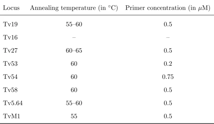
Table 2.2: Optimised PCR conditions for sevenamicrosatellite loci

Locus Annealing temperature (in ◦C) Primer concentration (in µM)

Tv19 55–60 0.5

Tv16 – –

Tv27 60–65 0.5

Tv53 60 0.2

Tv54 60 0.75

Tv58 60 0.5

Tv5.64 55–60 0.5

TvM1 55 0.5

a_{Locus Tv16 was excluded from the panel due to difficulties with PCR optimisation}

and its linkage to locus Tv27

2.2.4 Fragment Analysis

The products of microsatellite singleplex reactions were visualised on 1.5%

agarose gels to screen for positive bands, in the same fashion as described

in section 2.2.2. Those products that exhibited strong positive bands were

selected for capillary electrophoresis.

Capillary electrophoresis was carried out using an ABI PRISM 3130xl

sequencer (Applied Biosystems). Products were submitted on a 96-well

micro-plate. Each well contained 0.5 µL of PCR product, 12 µL of

Hi-Di formamide (Applied Biosystems) and 0.3 µL of GeneScan–500 LIZ size

standard (Applied Biosystems). In some cases, when PCR products showed

weak bands on agarose gel electrophoresis, 1 µL of product was added to

the mixture. The micro-plate was sealed and the mixture in the wells was

denatured for 1 min at 95◦C. In order to prevent re-annealing of DNA

(41)

the sequencer.

Allele scoring

Fragments were visualised and their sizes estimated using Peak Scanner

v1.0 (Applied Biosystems). A combined results table was then exported

in .txt format into the program MICROSATELIGHT (Palero et al. 2011).

This program is an open-source platform specifically developed to score

mi-crosatellite data and translate its outputs into files that can be interpreted

by a variety of commonly used population genetics software.

MICROSATELIGHT offers automated and manual possibilities for

defin-ing allele bin boundaries (AlleloBin, Prasanth et al. 2006; Binator, Palero

et al. 2011). Binning was performed using the AlleloBin sub-routine.

Al-leloBin implements the least square minimisation algorithm defined by Idury

& Cardon (1997).

In order to detect all of the alleles produced during PCR reactions,

al-lele scoring was completed by visually inspecting all electropherograms and

comparing these observations with results from automated allele scoring.

2.2.5 Genotyping error

In order to detect and quantify the magnitude and frequency of genotyping

error, a minimum of two samples per locality were randomly selected for

replication (n = 8). The selected samples represent ∼ 20% of the total

dataset as advised by (Pompanon et al., 2005). Microsatellite amplification

(42)

2.2.6 Data Analysis

Microsatellite polymorphism

The number of alleles per locus, number of private alleles, observed (Ho),

and the expected heterozygosity (He) were estimated for each locus across

localities. In order to detect deviations from Hardy-Weinberg expectations

(HW), a HW equilibrium test was performed. Because there was noa priori

expectation of heterozygote excess or deficit, an HW exact probability test

was chosen (Guo & Thompson, 1992; Weir, 1996). Wright’s F statistics,

such as the inbreeding (Fis) and subpopulation structure coefficients (Fst),

were estimated using the analysis of variance (ANOVA) framework defined

in Weir & Cockerham (1984) and Weir (1996). Fst was favoured over other

measures of population structure, such asRst, because it performs relatively

well for moderately structured populations, when a small number of loci is

analysed, and is independent of microsatellite mutation patterns (Holsinger

& Weir, 2009; Balloux & Lugon-Moulin, 2002). An exact test of population

differentiation (100000 Markov chain steps Goudet et al., 1996; Raymond

& Rousset, 1995) was performed to determine whetherFst among localities

significantly differs from zero.

Genetic diversity measures were estimated with the program GENALEX

(Peakall & Smouse 2006), which is built into Microsoft Exel. The HW

exact probability tests and F statistics were estimated using GENEPOP

v.4.1.1 (Rousset, 2008). It is worth noting that Rousset (2008) implemented

slight modifications to the estimation ofF statistics in the latest version of

GENEPOP. Details of these modifications can be found in Rousset (2008).

Both the Fis and Fst goodness of fit tests were performed in the program

(43)

Probability of identity

In order to quantify the panel’s ability to discriminate individuals, allele

fre-quencies of each locus were used to estimate the probability of identity (P I).

Because the dataset in this study is likely to contain related individuals (a

violation of one of the fundamental assumptions for an unbiased calculation

ofP I) the panel’s discriminatory power was estimated using the more

con-servative probability of identity adjusted for siblings (P Isib). P Isibaccounts

for potential underestimation ofP Iand was estimated by the formulae given

in Taberlet & Luikart (1999) and Waits et al. (2001).

The per locus P Isib is given by the equation:

P Isib= 0.25 + (0.5

X

p2_i) + [0.5(Xp2_i)2]−0.25(Xp4_i) (2.1)

where the termpi is the allele frequency of theith allele at a given locus.

In accordance with the product rule, the multi-locusP Isibis obtained by

multiplying theP Isibvalues of each individual locus. The effect that

remov-ing a particular locus would have on the discriminatory power of the panel

was evaluated by re-estimating theP Isibiteratively, excluding the

informa-tion from one locus on each occasion. These calculainforma-tions were performed in

the program GENALEX.

Genotyping error

Genotyping errors were detected by comparing the multi-locus genotype of

blindly replicated samples with their corresponding multi-locus genotype in

the original dataset. To avoid further ambiguities only allele size estimates

prior to binning were compared.

(44)

main classes: 1) stochastic errors, which include allelic drop-out and false

alleles; and 2) systematic errors, which cover scoring errors, contamination

and sample confusion. False alleles were scored only when differences

be-tween replicated alleles were equal to or greater than two base pairs. Data

on the prevalence of stochastic errors was used to estimate per locus allele

drop-out rate (pl), per locus false allele rate (fl), weighted average of allele

drop-out rate (pw) and weighted average of false allele rate (fw), according

to the equations defined in Broquet & Petit (2004).

In order to have a more general metric for error quantification, the mean

error rate per locus (el) and the observed error rate per multi-locus

geno-type (eobs) were estimated with the equations given in Pompanon et al.

(2005). These equations require counting the frequency of mismatches. A

mismatch was scored when a minimum of one allele on each locus differed

from the corresponding alleles in the reference genotype. Only mismatches

correspondent to stochastic and scoring errors were taken into account to

estimateelandeobs, since mismatches associated with contamination or

sam-ple swapping are not the direct result of locus or reaction characteristics. It

was considered that systematic errors can be mitigated by an increased level

of training and by enforcing more stringent laboratory and data handling

protocols.

To assess if any deficit in heterozygotes is compatible with the

pres-ence of null alleles across loci, the tests implemented by the program

MI-CROCHECKER (van Oosterhout et al. 2004) were applied to data from the

(45)

2.3 Results

2.3.1 Sample characteristics

A total of 37 individuals were captured and sacrificed. Of these, 20 were

male, 14 were female and 3 were pouch-young of undetermined sex. Except

for the 3 pouch young individuals, it was impossible to determine a priori

if all of the adult individuals collected in this study were related.

Fur colouration of 16 individuals was categorised as black while 17 were

categorised as grey. There were four individuals who were skinned before

fur colouration pattern could be determined. A great deal of variation in

fur tones was noted, thus the categorisation is considered subjective and is

provided as supplementary information only.

2.3.2 DNA quantification and screening

Tissue samples yielded variable but relatively high DNA concentrations.

A total of 71 extractions were necessary to ensure the freshness of

tem-plate DNA used for optimisation reactions. The first batch of extractions,

corresponding to 37 individuals, was performed between June-July of 2011

(median = 59.85 ng/µL, range: 29.11–297.03 ng/µL; Figure 2.2). A second

batch of just 34 individuals was extracted during October 2011 (median =

57.22 ng/µL, range: 22.61–168.00 ng/µL). All extracts exhibited positive

bands for CO-I region amplification.

2.3.3 Microsatellite amplification

PCR conditions for seven out of eight microsatellite primer pairs were

op-timised allowing for the generation of multi-locus genetic profiles of the 37

(46)

con-2.3. RESULTS 29

Figure 2.2: DNA concentration measured in ng/µL. Bars represent tissue

samples from which DNA was extracted between June-July, 2011. The

horizontal line represents the median DNA concentration (59.85 ng/µL)

ditions for marker Tv16 could not be optimised, thus forcing its exclusion

from the panel. The automated algorithm implemented to assign raw

al-lele size lengths into discrete size categories performed well for all markers

examined in this study, as revealed by the low magnitudes of normalised

variance estimated during the binning process (Idury & Cardon, 1997, data

not shown).

All refined loci showed moderate levels of allelic diversity except for locus

Tv54, which showed a reduced number of alleles across localities (Figure 2.3).

Most alleles detected in the study were present across all of the sampled sites,

although there were some instances in which private alleles were detected.

This is the case for the Lewis Pass sample site, which despite having a

reduced sample size compared to Hororata, showed a greater prevalence of

(47)

Figure 2.3: Number of alleles observed across loci and location in Can-terbury. Numbers on the x-axis represent the different loci in ascending order as follows: 1= Tv19, 2 = Tv27, 3 = Tv53, 4 = Tv54, 5 = Tv58, 6 = Tv5.64 and 7 = TvM1

Banks Peninsula (Table 2.3).

Despite a low mean sample size (mean ± SE: 12.29 ± 1.04), it was

possible to detect moderate levels of allelic diversity (5.57 ± 0.5) and

ob-served heterozygosity (0.64 ± 0.06) across localities. As expected by the

number of alleles detected, locus Tv54 was the only one in which observed

heterozygosity levels were low across all localities. Locus Tv58 exhibited

low heterozygosity levels both in Hororata and Banks Peninsula, while

(48)

2.3. RESULTS 31

(Table 2.3).

From the three localities sampled in this study, Hororata (χ2 _{= 33.98;}

d.f. = 14; P = 0.0021) and Lewis Pass (χ2 = 23.11; d.f. = 12; P = 0.026)

showed significant departures from HW equilibrium. When results of the

exact probability tests were partitioned in locus/locality combinations, six

out of twenty one combinations showed significant departures from HW

ex-pectations (Table 2.4). However, after the sequential Bonferroni correction

was applied (Holm, 1979), only locus Tv58 in Hororata exhibited significant

departures from HW expectations (P = 0.019).

Loci evaluated in this study showed a low proportion of genetic diversity

due to allele frequency differences among localities (Fst = 0.03). However,

a detailed partition of Fst parameters revealed moderate levels of genetic

structure for locus Tv19 (Table 2.3). Evidence of lack of genetic structure

was further supported by a pairwise comparison matrix ofFst (Table 2.5).

From Table 2.5 it is possible to visualise Fst magnitudes among localities

indicating only moderate to low structuring. Finally, the exact test of

pop-ulation differentiation showed that the overall value ofFst found among the

three localities does not significantly differ from zero (P = 0.179).

2.3.4 Probability of identity

TheP Isibestimated on the basis of allele frequencies for all localities sampled

in Canterbury was 3.0×10−3. This parameter indicates that the

microsatel-lite panel optimised in the present study provided sufficient information to

identify individual possums based on their multi-locus genetic profile. When

this parameter was re-estimated by separating allele frequencies per sampled

site, some variation in the magnitude ofP Isibwas observed (Figure 2.4).

(49)

(50)

2.3. RESULTS 33

Table 2.4: Summary of statistical parameters estimated per locus at each of

the localities sampled in Canterbury. The HWexact probability testP-values

(HWP)a and their standard error (SE) as well as theP Isibfor every locus are

presented in this table

Banks Peninsulab Hororatac Lewis Passd

Locus HWP SE P Isib HWP SE P Isib HWP SE P Isib

Tv19 0.013 0.000 0.476 0.007 0.001 0.459 0.01 0.00 0.369

Tv27 0.310 0.016 0.386 0.279 0.016 0.366 0.16 0.02 0.338

Tv53 0.537 0.022 0.369 0.390 0.021 0.397 0.01 0.00 0.366

Tv54 1.000 0.000 0.899 0.720 0.000 0.638 NA NA 1.000

Tv58 0.034 0.006 0.665 0.000 0.000 0.462 0.65 0.03 0.454

Tv5.64 0.779 0.000 0.506 0.469 0.012 0.455 1.00 0.00 0.436

TvM1 1.000 0.000 0.387 0.832 0.008 0.379 0.79 0.01 0.370

a

P-values before sequential Bonferroni correction are presented here

b

Banks PeninsulaP Isib= 7.9×10−3

c

HororataP Isib= 3.4×10−3

d