Proceedings of the 56th Annual Meeting of the Association for Computational Linguistics (Long Papers), pages 527–536 527
Context-Aware Neural Model for Temporal Information Extraction
Yuanliang Meng Text Machine Lab for NLP Department of Computer Science University of Massachusetts Lowell
Anna Rumshisky Text Machine Lab for NLP Department of Computer Science University of Massachusetts Lowell
Abstract
We propose a context-aware neural net-work model for temporal information ex-traction, with a uniform architecture for event-event, event-timex and timex-timex pairs. A Global Context Layer (GCL), inspired by the Neural Turing Machine (NTM), stores processed temporal rela-tions in the narrative order, and retrieves them for use when the relevant entities are encountered. Relations are then clas-sified in this larger context. The GCL model uses long-term memory and atten-tion mechanisms to resolve long-distance dependencies that regular RNNs cannot recognize. GCL does not use postprocess-ing to resolve timegraph conflicts, outper-forming previous approaches that do so. To our knowledge, GCL is also the first model to use an NTM-like architecture to incorporate the information about global context into discourse-scale processing of natural text.
1 Introduction
Extracting information about the order and timing of events from text is crucial to any system that attempts an in-depth natural language understand-ing, whether related to question answerunderstand-ing, ral inference, or other related tasks. Earlier tempo-ral information extraction (Tempotempo-ralIE) systems tended to rely on traditional statistical learning with feature-engineered task-specific models, typ-ically used in succession (Yoshikawa et al.,2009;
Ling and Weld,2010;Sun et al.,2013;Chambers et al.,2014;Mirza and Minard,2015).
Recently, there have been some attempts to ex-tract temporal relations with neural network mod-els, particularly with recurrent neural networks
(RNN) models (Meng et al., 2017; Cheng and Miyao, 2017; Tourille et al., 2017) and convolu-tional neural networks (CNN) (Lin et al., 2017). These models predominantly use token embed-dings as input, avoiding handcrafted features for each task. Typically, neural network models out-perform traditional statistical models. Some stud-ies also try to combine neural network models with rule-based information retrieval methods (Fries,
2016). These systems require different models for different pair types, so several models must be combined to fully process text.
A common disadvantage of all these models is that they build relations fromisolated pairs of entities (events or temporal expressions). This context-blind, pairwise classification often gener-ates conflicts in the resulting timegraph. Common ways of ameliorating the conflicts is to apply some
ad hocconstraints to account for basic properties of relations (e.g. transitivity), often without con-sidering the content of the text per se. For ex-ample, Ling and Weld (2010) designed transitiv-ity formulae, used with local features.Sun(2014) proposed a strategy that “prefers the edges that can be inferred by other edges in the graph and remove the ones that are least so”. Another approach is to use the results from separate classifiers to rank re-sults according to their general confidence (Mani et al.,2007;Chambers et al.,2014). High-ranking results overwrite low-ranking ones. Meng et al.
memory as “context” for further processing. If the later evidence suggests our early interpretation was wrong, we can correct it.
This paper proposes a model to simulate such mechanisms. Our model introduces a Global Con-text Layer (GCL), inspired by the Neural Turing Machine (NTM) architecture (Graves et al.,2014), to store processed relations in narrative order, and retrieve them for use when related entities are en-countered. The stored information can also be up-dated if necessary, allowing for self-correction.
This paper’s contributions are as follows. To our knowledge, this is the first attempt to use neu-ral network models with updateable external mem-ory to incorporate global context information for discourse-level processing of natural text in gen-eral and for temporal relation extraction in par-ticular. It gives a uniform treatment of all pairs of temporally relevant entities. We obtain state-of-the-art results on TimeBank-Dense, which is a standard benchmark for TemporalIE.
2 Dataset
We train and evaluate our model on TimeBank-Dense1 (Chambers et al., 2014). There are 6 classes of relations: SIMULTANEOUS, BEFORE, AFTER, IS INCLUDED, INCLUDES, and VAGUE TimeBank-Dense annotation aims to approximate a complete temporal relation graph by including all intra-sentential relations, all relations between adjacent sentences, and all relations with docu-ment creation time. TimeBank-Dense is one of the standard benchmarks for intrinsic evalution of TemporalIE systems. We follow the experimental setup inChambers et al. (2014), which splits the corpus into training/validation/test sets of 22, 5, and 9 documents, respectively. Previous publica-tions often use the micro-averaged F1 score, which is equivalent to accuracy in this case. We also rely on the micro-averaged F1 score for model selec-tion and evaluaselec-tion.
FollowingMeng et al.(2017), we augment the data by flipping all pairs, except for relations in-volving document creation time (DCT). In other words, if a pair (ei, ej) exists, we add (ej, ei) to
the dataset with the opposite label (e.g. BEFORE becomesAFTER). The augmentation applies to the validation and test sets also. In the final evaluation, a double-checking technique picks one result from
1https://www.usna.edu/Users/cs/
nchamber/caevo/#corpus
the two-way classification, based on output scores. The dataset is heavily imbalanced. The training set has as much as 44.1%VAGUElabels, whereas only 1.8% labels areSIMULTANEOUS. We did not do any up-sampling or down-sampling.
3 System
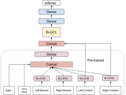
[image:2.595.311.524.312.473.2]Our system has two main components. The first one is a pairwise relation classifier, and the other is the Global Context Layer (GCL). The pairwise re-lation classifier follows the architecture designed byMeng et al.(2017), which used the dependency paths to the least common ancestor (LCA) from each entity as input. We train the first component first, and then assemble them in a combined neu-ral network to continue training. Fig. 1gives an overview of the system.
Figure 1: System overview. Originally, the pre-trained sys-tem has one more dense layer and an output layer, but they are truncated before combination. The max pooling layers on top of each Bi-LSTM layers are omitted here.
3.1 Global Context Layer
The Global Context Layer (GCL) we propose is inspired by the Neural Turing Machine (NTM) ar-chitecture, which is an extension of a recurrent neural network with external memory and an at-tention mechanism for reading and writing to that memory. NTM has been shown to perform ba-sic tasks such as copying, sorting, and associative recall (Graves et al., 2014). The external mem-ory not only enables a large (theoretically infinite) capacity for information storage, but also allows flexible access based on attention mechanisms.
canoni-cal NTM, it is more suitable for the task of retain-ing and updatretain-ing global context information.
3.1.1 Motivation
Vanilla RNNs struggle with capturing long-distance dependencies. Gated RNNs such as LSTM have trainable gates to address the “van-ishing and exploding gradient” problem ( Hochre-iter and Schmidhuber,1997). At each time step, it chooses what to memorize and forget, so patterns over arbitrary time intervals can be recognized. However, the memory in LSTM is stillshort-term. No matter how long the cell states keep certain in-formation, once it is forgotten, it gets lost forever. Such a mechanism suffices for modeling contigu-ous sequences. For example, sentences are nat-urally fit units for such models, since a sentence starts only after the preceding sentence is finished, and LSTM may be an adequate tool to process sen-tences. However, when the sequences are not con-tiguous, as in temporal and other discourse-scale relations, LSTM models do not have the capabil-ity to look for input pieces across sequences.
When humans read text, discourse-level infor-mation is often distributed across the full scope of the text. To fully understand an article, we must be able to organize the processed information across sentences and paragraphs. In particular, to inter-pret temporal relations between entities in a sen-tence, sometimes we also look at relations with other entities elsewhere in the text. Such entities or relations form no regular sequences, and only a system with long-term memory as well as atten-tion mechanisms can process them. An NTM-like architecture has an external memory with attention mechanisms, so it is an ideal candidate for such tasks. Furthermore, unlike the models that use at-tention over inputs (Vinyals et al., 2015; Kumar et al.,2016), NTM-like models are capable of up-dating previously stored representations. We de-scribe below the GCL architecture that we use to store and update the global context information.
3.1.2 Reading
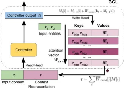
[image:3.595.308.526.65.218.2]The input to the GCL layer is a concatenation of three layers from the pairwise neural network. Two of these are the entity context representation layers, encoded by the two LSTM branches. The other is the penultimate hidden layer before the output layer, which encodes the relation. We can write them as[e1,e2,x]. The context representa-tions are used as “keys” to uniquely identify the
Figure 2: GCL computing attention weights. Input entity rep-resentations are compared to the Key section of GCL mem-ory. Slots with the same or similar entities get more attention.
entities. Note that we use flat context embeddings, rather than dependency path embeddings, because dependency paths tend to be short and will also vary for the same entity, depending on the other entity in the pair. As such, they do not provide a unique way to represent an entity.
The original design of NTM has a complex addressing mechanism for reading, which also makes it difficult to train. An important difference in GCL is that we separate the “key” component from the “content” component of memory. Each memory slot S[i]consists of [K[i];M[i]], where S is the whole memory withnslots,i ≤nis the index, K is the key and M is the content. Ad-dressing is only performed on the key component. The key component stores the representation of two entities, provided by the layers encoding the flat entity context.
K[i] =eM1[i]⊕eM2[i] (1)
Here⊕is the concatenation operator. In the GCL model, the read head computes a reading weight Wn×1from the input entity representationse1,e2 and the entity representationseM1,eM2in mem-ory (i.e., the keys in each memmem-ory slot). The first step is to compute the distance between current in-put and the memory columns, as shown in Eq.2. D[i]is the Euclidean distance between the input key and the memory key of slot M[i]. D0[i] is computed after flipping the two entities. We do so because the order of entities in a pair should not affect their relevance.
D[i] =1
Z||e1⊕e2−eM1[i]⊕eM2[i]||
2 2
D0[i] =1
Z0||e2⊕e1−eM1[i]⊕eM2[i]||
2 2
where Z = P
iD[i]is the normalization factor,
and so is Z0 for the flipped case. The reading weight is then calculated as in Eq.3, where1n×1
is a vector of all 1’s.
W[i] = max(softmax(1−D)[i],
softmax(1−D0)[i]) (3)
Every element of W represents the relevance of the corresponding memory slot (see Fig.2). Often it is still too blurred and needs to be further sharp-ened as in Eq.4. Hereβis a positive number.Wβ is a point-wise exponential function by power of β. A largeβallows “winner takes all”, so only the most relevant memory slots are read.
Wread = softmax(Wβ) (4)
Parameterβcould be a constant, or could be traable. Our model computes it from the current in-put xt and the previous output ht−1, and thus it
varies in each time step. Wsharp and bsharp are
trainable weights and bias, cβ is a constant, and
ReLU is the rectified linear function.
βt=ReLU(Wsharp[xt,ht−1]+bsharp)+cβ (5)
With the sharpened reading weight vector, we are able to obtain the read vector r1×m fromM as a
weighted sum, as in Eq.6.
r=X
i
Wread[i]M[i] (6)
Generally speaking, the depth of memory M should be large enough to allow sparse encoding, so that crucial information is not lost after the sum-mation. The read vector then contains contextual information relevant to current input. Both the read vector and the current input are fed to the con-troller, yielding GCL output. Unlike the canonical NTM, the CGL model does not have a trainable gate interpolating theWtcomputed at timet, with
Wt−1computed at previous timet−1. The weight
vector is not passed to next time step, so the atten-tion has no “inertia”.
We tried two variants of the controller: (a) state-tracking, with an LSTM layer, and (b) stateless, with a dense layer. An LSTM controller has an internal state, and also has gates to select input and output. If the input data and/or the read vec-tor from M have regular patterns with respect to time steps, an LSTM controller would be a better choice. For the specific task of temporal relation extraction, we saw no difference in performance.
3.1.3 Writing
The controller produces an output ht, which is
sent to the next layer and also used to updateM. Similar to reading, the first step of writing pro-cedure is to compute an attention weight vector over the slots ofM. As described above, the read-ing procedure computes a weighted sum over slots of M. The writing procedure writes a weighted ht to each slot. The attention mechanism here is de factoa soft addressing mechanism. The slots with a higher attention value will be the addresses which will get more of an update.
The same weight vectorW computed as shown in Eq. 3 is used for writing. However, an addi-tional operation is introduced for writing. Recall that the weights are computed from entity repre-sentations. If the input entities aree1 ande2, the weight vector should have high values in the slots corresponding to e1 and/or e2. But we may not always want relevant memory slots to be overwrit-ten. Instead, additional information can be written to a different slot. Additionally, whenM is rela-tively empty, as at the beginning, the addressing mechanism may treat all slots equally, and uni-formly update all slots in the same way. In this case we want the weight vector to shift each time, soMcan diversify fast.
Therefore we use a shift function similar to the canonical NTM. The idea is to compute a shifted weight vector Wf by convolving W with a shift
kernelswhich maps a shift distance to a probabil-ity value. For example,s(−1) = 0.2,s(0) = 0.5,
s(1) = 0.3means the probabilities of shifting left, no shifting, and shifting right are 0.2, 0.5, 0.3, re-spectively. Generally speaking, we wantsto give zeros for most shift distances, so the shifting oper-ation is limited to a small range.
f
W[i] =
n−1
X
j=0
W[j]s[i−j] (7)
At each time step, the shift kernel depends on cur-rent input and output. If the allowed shift range is [-s/2, +s/2], we train a weight Ws and biasbs to
calculate the shift weightsCs×1,
Ct= softmax(Ws[xt,ht] +bs) (8)
Then the weights are mapped to a circulant ker-nel to perform the convolution in Eq.7, the final output isWf.
shifting are “soft” in nature, and thus could yield a blurred outcome. Again, we train the weights to obtain a sharpening parameterγeach time, and perform softmax overWf.
γt=ReLU(Wsharp[xt,ht] +bsharp) +cγ (9)
Wwrite= softmax(Wfγ) (10)
f
Wγ is the point-wise exponential function, over the shifted weight vector.cγis a positive constant.
The original NTM model has gates for interpo-lating Wfγ at the current time with the one
com-puted at the previous time step, but we omit this operation. We also omit theerase vector and the
add vector, soWwritefully controls what to
over-write in M and what to retain. As a result, the writing operation can be expressed as:
Mt[i] =Mt−1[i]+Wwrite[i](ht−Mt−1[i]) (11)
The first term in Eq.11is the memory in the pre-vious time step, and the second term is the update. We update the keys in the same way. As we can see, the keys come from entity representations, but are not exactly the same, due toWwrite.
Kt[i] =Kt−1[i] +Wwrite[i](e1⊕e2−Kt−1[i])
(12)
3.1.4 GCL vs. Canonical NTM
We highlight below some major differences be-tween the canonical NTM and the GCL model. Typically, NTM computes the keys from input and output for accessing different memory addresses. In GCL, the keys are simply the entity representa-tions[e1,e2]from input, in either order. The key function effectively involves slicing and flipping the input. Further discussion of the differences be-tween the GCL addressing mechanism and some of the other NTM variations is provided in Sec.5. Another major difference is that we do not use any gates to interpolate the attention vector at the current time step with the one from the previous time step. Instead, the previous attention vector is totally ignored. Since we do not compute the erase vector or the add vector, this allows the attention vector to fully control memory updates.
In addition, we unified the trainable weights for calculatingβ andγ at each time step. We found these parameters not to be crucial, and setting them to be constant does not affect the results. We also do not shift attention for reading. A possible
advantage of shifting attention is that neighboring slots of the focus can also be accessed, providing a way to simulate associative recall. This is based on the fact that the writing procedure tends to write similar memories close to each other. However, in this study we want the reading procedure to be re-stricted. Associative recall can be realized from attention vector itself, without shifting.
3.2 Pairwise Classification Model
The pairwise model classifies individual entity pairs, where entities are events and time expres-sions (timexes). In other words, for each pair, we only use the local context, and the relation of one pair does not affect the classification results for other pairs. We follow the architecture pro-posed inMeng et al.(2017), but with the follow-ing changes: (1) all three types of pairs are han-dled by the same neural network, rather than by three separately trained models; (2) the neighbor-ing words (a flat context) of entity mentions are used to generate input, in addition to words on syntactic dependency paths; (3) all timex-timex pairs are included as well, not only event-timex and event-event pairs; (4) every pair is assigned a 3-dimensional “time value”, to approximate the rule-based approach when possible.
3.2.1 Event Pairs and Event-Timex Pairs
TimeBank-Dense dataset labels three types of pairs: intra-sentence, cross-sentence and docu-ment creation time (DCT). For intra-sentence pairs and cross-sentence pairs, we follow Meng et al.
(2017). The shortest dependency path between the two entities is identified, and the word embeddings from the path to the least common ancestor for each entity are processed by two LSTM branches, with a separate max pooling layer for each branch. Path to the root is used for cross-sentence rela-tions. For relations with the DCT, we use a single word now as a placeholder for the DCT branch. UnlikeMeng et al.(2017), we allow the model to accept all three pair types, with a “pair type” fea-ture as a component of input, defined as an integer with the value 1, -1 or 0, respectively.
In addition to the shortest dependency path, our model also uses a flat local context window, that is, the words around each entity mention, regard-less of syntactic structures. For an entity start-ing with word wi, the local context window is
short at the edge of a sentence, or when the sec-ond entity in encountered. By using this context window, the words between two entities are of-ten used twice by the system, and thus given more consideration. To inform the system of other en-tity mentions, we also add special input tokens at the locations where events and timexes are tagged. The embeddings of the special tokens are uni-formly initialized, and automatically tuned during the training process.
3.2.2 Timex Pairs
The method described inMeng et al.(2017) clas-sifies timex pairs by handcrafted rules and then adds them to the final results prior to postprocess-ing. Since timexes have concrete time values, a rule-based method would seem appropriate. How-ever, since our model uses global context to help classify relations and timex-timex pairs enrich the global context representation, we design a way for a common classifier model to handle such pairs.
When DCT is not involved, timex pairs are cre-ated the same way as cross-sentence pairs, that is, path to the root is used for each entity. DCT is represented by the placeholder wordnow. In ad-dition to the word-based representations, another input vector is used to simulate the rule-based ap-proach, to be explained next.
3.2.3 Time Value Vectors
Every timex tag has a time value, following the ISO-8601 standard. Every value can be mapped to a 2D vector of real values(start, end). For a pair we use the subtraction of the vectors to represent the difference. Suppose we have timexes in below:
THE HAGUE, Netherlands (AP)_ The World Court <TIMEX3 tid="t21" type="DATE" value="1998-02-27" temporalFunction="true" functionInDocument="NONE" anchorTimeID="t0">Friday</TIMEX3> rejected U.S. and British objections to a Libyan World Court case that has the trial of two Libyans suspected of blowing up a Pan Am jumbo jet over Scotland in <TIMEX3 tid="t22" type="DATE" value="1988" temporalFunction="false"
functionInDocument="NONE">1988</TIMEX3>.
The first timex can be represented as (1998 + 1/12 + 26/365, 1998 + 1/12 + 26/365) = (1998.155, 1998.155), and the second one (1988, 1988 + 364/365) = (1988, 1988.997). The difference of the values are put in the sign function, to ob-tain the representation: (sign(1988 - 1998.155), sign(1988.997 - 1998.155)) = (-1, -1). Vector (-1, -1) clearly indicates the AFTER relation between t21andt22. We set the minimum interval to be a day, which is generally sufficient for our data. The
DURATIONtimexes are not considered, and word-based input vectors are used to represent them.
In order to make all the input data have the same shape, we assign the time value vector to all pairs, even if a timex is not involved. For non-timex pairs, a vector (-1, 0, 0) is used. The first element -1 to indicate a “pseudo” time value. Real timex pairs have the first value of 1, so the example we just discussed would be assigned a vector (1, 1, -1). The time value vectors allow the model to take advantage of rule-based information.
3.3 Combining Two Components
We tried training the two components in a com-bined system, but found it slow to converge. In our experiments, we trained the pairwise model first, froze it, and then combined it with the GCL layer to train the GCL. This method also helps us ob-serve whether the GCL component alone improves results, given the same input.
We tried combining the systems in two ways. One is to connect the output layer of the pre-trained model to GCL, and the other is to slice the pre-trained model and connect its hidden layer to GCL. All the GCL layers are bi-directional, aver-aging forward and backward passes. By connect-ing the output layer, which has a softmax activa-tion, we hand the final decisions made by the pair-wise model to GCL. On the other hand, the hid-den layer provides higher layers with cruder but richer information. We found that the latter per-forms better. It is also possible to train the two components together from scratch. In this case, the learning rate has to be set much lower to as-sure convergence, and the training requires more epochs.
4 Experiments
For all the experiments, hyperparameters includ-ing the number of epochs are tuned with the val-idation set only. Training data is segmented into chunks. Each chunk contains relation pairs in the narrative order. The size of chunks is randomly chosen from [40, 60, 80, 120, 160] at the begin-ning of each epoch of traibegin-ning. The GCL main-tains a memory for each chunk, and clears it at the end of a chunk. The idea here is to train the model on short paragraphs to avoid overfitting.
2, chunkiwill start with pairni+chunksize+11.
11 is a prime number we chose to assure each epoch observes different compositions of chunks. By doing the rotation, some pairs in the final chunk of epoch 1 will show up in the first chunk in epoch 2 as well. However, within each chunk, we do not randomize pairs, so narrative order is preserved at this level. We also do not shuffle the chunks, but only rotate them.
Evaluation on the test set uses only one chunk for each file (chunk size is the number of pairs). Each relation pair is only processed once, without “multiple rounds of reading”. Thus, we essentially train the model to read shorter paragraphs (varied in length), but test it on long articles.
4.1 Pairwise Model
As described in Section 3.2, the pairwise classi-fier has the following input vectors: left and right shortest path branches, two flat context vectors, a pair type flag, and a time value vector. Word em-beddings are initialized with glove.840B.300d word vectors2, and set to be trainable. The Bi-LSTM layers are followed by max-pooling. The two hidden layers have size 512 and 128, respec-tively. We train this model for 40 epochs, us-ing the RMSProp optimizer (Tieleman and Hin-ton, 2012). The learning rate is scheduled as lr = 2×10−3 ×2−n
5, where n is the number
of epochs.
The middle block of Table 1 shows the per-formance of the pairwise model after applying double-checking. Since all pairs are flipped, double-checking combines results from (ei, ej)
and (ej,ei), picking the label with the higher
prob-ability score, which typically boosts performance. The results without double-checking show similar trends.
4.2 GCL model
After training the pairwise model, we combine it with GCL. Unless otherwise indicated, the results reported in this section use the model configura-tion that connects the hidden layer (rather than the output layer) of the pairwise model with a bidirec-tional GCL layer. The bidirecbidirec-tional GCL is real-ized as the average of a forward GCL and a back-ward GCL, each producing a sequence. Then two more hidden layers are put on top of it, followed
2
https://nlp.stanford.edu/projects/glove/
3This result does not include timex-timex pairs, which is
3% of total test instances.
Model Micro-F1 Macro-F1
CAEVO (not NN model) .507
CATENA (not NN model) .511
Cheng et al. 2017 .5203
Meng et al. 2017 .519
pairwise .535 .528
Two more hidden layers .539 .532
GCL w/ state-tracking controller .545 .538
GCL w/ stateless controller .546 .538
[image:7.595.309.525.63.173.2]GCL w/ pre-trained output layer .541 .536
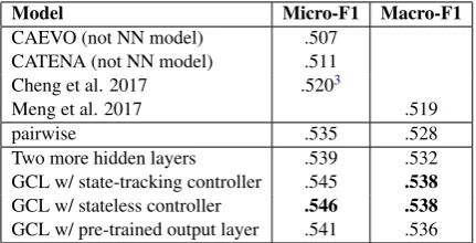
Table 1: Results on the test set. The GCL models use the same hyperparameters, if possible. The two models on the top do not use neural networks. The results in the two lower blocks all use double-check. “Two more hidden lay-ers” means adding two dense layers on top of the pre-trained model without using GCL. The last row corresponds to con-necting the output layer of a pre-trained model to GCL layers with stateless controller.
by an output layer. All the layers in the pre-trained pairwise model are set to be untrainable. The two trainable hidden layers have sizes 512 and 128, re-spectively, with ReLU activtion and 0.3 dropout after each one. The GCLs have 128 memory slots. Learning rate is scheduled aslr= 2×10−4×2−n2.
In the experiments, we found the models converge quite fast with respect to the number of epochs. It is not surprising because the lower layers are al-ready well trained, and frozen (no updating). Af-ter the 5th epoch, the training accuracy typically reaches 0.95. We stop training after 10 epochs.
The bottom block of Table 1 presents the re-sults, showing that all models from the present pa-per outpa-perform existing models from the literature. One may argue the combined system adds more hidden layers over a pre-trained model, which con-tributes to the improvement in performance. We show a comparison to a baseline model which adds two dense layers on top of the pairwise model, without the GCL. The configuration of the two layers is the same as we used for the GCL models. The result shows that the performance is slightly higher than what we get from the pairwise model, but the difference is smaller than what we get from GCL models – suggesting that the performance improvement with GCL models is not just due to more parameters. We also tried adding an LSTM layer on top of the pre-trained model, and found the system cannot converge. It again confirms that GCL is more powerful than LSTM in handling ir-regular time series.
pre-trained model to GCL seems to generate weaker results than connecting the hidden layer, although it also outperforms the pairwise model, and all pre-vious models in literature.
We performed significance testing to compare the pairwise model and the GCL-enabled model. A paired one-tailed t-test shows the results from the GCL model are significantly higher than re-sults from pairwise model (p-value 0.0015). While significant, the improvement is relatively small, we believe due in part to the small size of Timebank-Dense dataset.
4.3 Case Study
To illustrate the difference in performance of the pairwise model and the GCL model, we created a sample paragraph in which long-distance depen-dencies and references to DCT are needed to re-solve some of the temporal relations:
JohnmetMary in Massachusetts when theyattended the same university. They aregetting marriedin2019, 2 years after theirgraduation. Butthis year, they have relocatedto New Hampshire.
We created the gold standard annotation for this text with 5 events, 2 timexes, and 24TLINKs (see appendix)4. We set the DCT to an arbitrary date “2018-04-01”. There are noVAGUEor SIMULTA-NEOUSrelations.
For this paragraph, the pairwise model yields an accuracy (i.e. micro-averaged F1) of 0.292, while the GCL-enabled model yields 0.417. Overall, the GCL-enabled model assigns 6VAGUElabels while the pairwise assigns 11. It reflects the fact that GCL tries to infer relations from otherwise vague evidence. For example, it is difficult to infer the relation betweenmetand2019from the local con-text (without DCT, particularly), so the pairwise model labels it asVAGUE, while the GCL-enabled model correctly assignsBEFORE.
Recall that the GCL is placed on top of a pre-trained pairwise model, so the mistakes made by the pairwise model propagate to GCL. For exam-ple, the pairwise model incorrectly classifies2019
asBEFOREgraduation – perhaps, due to a some-what unusual syntax. But the GCL-enabled sys-tem assigns it aVAGUE label, probably as a way to compromise. In the TimeBank-Dense test data, VAGUE cases dominate, which may have made it more difficult for GCL to assign proper labels. In the future, we believe it may be better to omit
4Note that in TimeBank-Dense, no
TLINKSare associated
DURATIONtimexes, so 2 years is not annotated
writing (and reading) theVAGUErelations to/from GCL.
4.4 Error Analysis
Table 2 shows the overall performance for each relation using the GCL system with the stateless controller. Since we flip pairs and use double-checking to pick one result for each pair, BE-FORE/AFTER and IS INCLUDED/INCLUDES are actually treated in the same way, respectively. Here we map the results to original pairs, in order to compare to other systems.
Predicted labels
SIMUL BEF AFT IS INCL INCL VAG Total
SIMUL 10 0 9 2 1 17 39
BEF 0 327 27 15 5 215 589
AFT 1 26 208 4 5 184 428
IS INCL 1 27 3 59 2 67 159
INCL 0 16 9 2 19 70 116
VAG 1 171 87 28 17 596 900
Table 2: Overall results per relation.
As the table shows, the VAGUErelation causes the most trouble. It is not only because VAGUE is the largest class, but also because it is often semantically ambiguous, so even human experts have low inter-annotator agreement. If we allow a relatively sparse labeling of data, and use other evaluation methods (e.g. question answering), the VAGUEclass is not likely to have similar effects.
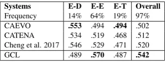
We also break down the results according to the types of pairs. Compared to other systems, our approach has a big advantage for event-event (E-E) pairs, which is by far the most common (64%) relation pairs for all data, and also requires more complex natural language understanding.
Com-Systems E-D E-E E-T Overall
Frequency 14% 64% 19% 97% CAEVO .553 .494 .494 .502 CATENA .534 .519 .468 .512 Cheng et al. 2017 .546 .529 .471 .520
[image:8.595.307.527.235.311.2]GCL .489 .570 .487 .542
Table 3: Results on the E-D, E-D and E-T pairs. GCL stands for the GCL-enabled system with a stateless controller. Frequencies are percentages in the test set. T-T pairs are not shown here. CAEVO is fromChambers et al.(2014). CATENA is fromMirza and Tonelli(2016)
[image:8.595.331.502.545.609.2]results, and found that the relatively low perfor-mance is mainly caused by misclassifyingVAGUE as AFTER. As Table 4 shows, among the 72
Predicted labels
SIMUL BEF AFT IS INCL INCL VAG SIMUL 0 0 0 0 0 0
BEF 0 57 11 15 6 37
AFT 0 3 36 0 0 10
IS INCL 0 11 1 31 1 12
INCL 0 0 2 1 3 2
[image:9.595.83.281.113.185.2]VAG 0 4 20 9 14 25
Table 4: Test results from event and document creation time (E-D) pairs. The rows are true labels and the columns are predicted labels.
VAGUErelations in E-D pairs, 20 are labeled AF-TERby our system. In a news article, most events occur before the DCT i.e. the time when the arti-cle was written. If the temporal relation is vague, our system tends to guess that the event occurs af-ter the DCT. It is inaf-teresting becauseAFTERonly accounts for 16% of all E-D pairs in test data (and about the same in training data), behind BEFORE (41%), VAGUE (21%), and IS INCLUDED(18%). However, E-D is a relatively small category with only 311 instances in the test set, so it is difficult to draw any a substantive conclusion in this case.
Recall that our model has a uniform architec-ture for all input types and is trained on event-event, event-timex and event-DCT pairs simulta-neously. As a result, its performance is not optimal for some lower-frequency pair types. Tuning the model for each pair type separately, as well as re-sampling to deal with class imbalance would, per-haps, improve performance. However, the point of these experiments was not to get the largest im-provement, but to show that the GCL mechanism can replace heuristic-based timegraph conflict res-olution, improving the performance of an other-wise very similar model.
5 Related Work
While the GCL model is inspired by NTM, other NTM variants have also been proposed recently.
Zhang et al. (2015) proposed structured memory architectures for NTMs, and argue they could alle-viate overfitting and increase predictive accuracy.
Graves et al. (2016) proposed a memory access mechanism on top of NTM, which they call Differ-entiable Neural Computer (DNC). DNC can store the transitions between memory locations it ac-cesses, and thus can model some structured data.
G¨ulc¸ehre et al. (2016) proposed a Dynamic Neural Turing Machine (D-NTM) model, which
allows discrete access to memory. G¨ulc¸ehre et al.
(2017) further simplified the addressing algorithm, so a single trainable matrix is used to get locations for read and write. Both models separate the ad-dress section from the content section of memory, as do we. We came up with the idea indepen-dently, noting that the content-based addressing in the canonical NTM model is difficult to train. A crucial difference between GCL and these mod-els is that they use input “content” to compute keys. In GCL, the addressing mechanism fully depends on the entity representations, which are provided by the context encoding layers and not computed by the GCL controller. Addressing then involves matching the input entities and the enti-ties in memory.
Other than NTM-based approaches, there are models that use an attention mechanism over ei-ther input or external memory. For instance, the Pointer Networks (Vinyals et al., 2015) uses at-tention over input timesteps. However, it has no power to rewrite information for later use, since they have no “memory” except for the RNN states. The Dynamic Memory Networks (Kumar et al., 2016) has an “episodic memory” module which can be updated at each timestep. However, the memory there is a vector (“episode”) with-out internal structure, and the attention mechanism works on inputs, just as in Pointer Networks. Our GCL model and other NTM-based models have a memory with multiple slots, and the addressing function (attention) dictates writing and reading to/from certain slots in the memory.
6 Conclusion
We have proposed the first context-aware neural model for temporal information extraction using an external memory to represent global context. Our model introduces a Global Context Layer which is able to save and retrieve processed tem-poral relations, and then use this global context to infer new relations from new input. The memory can be updated, allowing self-correction. Experi-mental results show that the proposed model beats previous results without resorting to ad-hoc reso-lution of timegraph conflicts in postprocessing.
Acknowledgments
References
Nathanael Chambers, Taylor Cassidy, Bill McDowell, and Steven Bethard. 2014. Dense event ordering with a multi-pass architecture. Transactions of the Association for Computational Linguistics, 2:273– 284.
Fei Cheng and Yusuke Miyao. 2017. Classifying tem-poral relations by bidirectional lstm over depen-dency paths. InACL.
Jason Alan Fries. 2016. Brundlefly at semeval-2016 task 12: Recurrent neural networks vs. joint infer-ence for clinical temporal information extraction. CoRR, abs/1606.01433.
Alex Graves, Greg Wayne, and Ivo Danihelka. 2014.
Neural turing machines.CoRR, abs/1410.5401.
Alex Graves, Greg Wayne, Malcolm Reynolds,
Tim Harley, Ivo Danihelka, Agnieszka Grabska-Barwinska, Sergio Gomez Colmenarejo, Edward Grefenstette, Tiago Ramalho, John Agapiou, Adri`a Puigdom`enech Badia, Karl Moritz Hermann, Yori Zwols, Georg Ostrovski, Adam Cain, Helen King, Christopher Summerfield, Phil Blunsom, Koray Kavukcuoglu, and Demis Hassabis. 2016.
Hybrid computing using a neural network with dynamic external memory. Nature, 538(7626):471– 476.
C¸ aglar G¨ulc¸ehre, Sarath Chandar, and Yoshua Bengio. 2017. Memory augmented neural networks with wormhole connections.CoRR, abs/1701.08718.
C¸ aglar G¨ulc¸ehre, Sarath Chandar, Kyunghyun Cho, and Yoshua Bengio. 2016. Dynamic neural tur-ing machine with soft and hard addresstur-ing schemes. CoRR, abs/1607.00036.
Sepp Hochreiter and J¨urgen Schmidhuber. 1997. Long short-term memory. Neural Computation, 9(8):1735–1780.
Ankit Kumar, Ozan Irsoy, Peter Ondruska, Mohit Iyyer, James Bradbury, Ishaan Gulrajani, Victor Zhong, Romain Paulus, and Richard Socher. 2016.
Ask me anything: Dynamic memory networks for natural language processing. InProceedings of The 33rd International Conference on Machine Learn-ing, volume 48 ofProceedings of Machine Learning Research, pages 1378–1387, New York, New York, USA. PMLR.
Chen Lin, Timothy A. Miller, Dmitriy Dligach, Steven Bethard, and Guergana Savova. 2017. Representa-tions of time expressions for temporal relation ex-traction with convolutional neural networks. In BioNLP 2017, Vancouver, Canada, August 4, 2017, pages 322–327.
Xiao Ling and Daniel S. Weld. 2010. Temporal infor-mation extraction. In Proceedings of the Twenty-Fourth AAAI Conference on Artificial Intelligence, AAAI 2010, Atlanta, Georgia, USA, July 11-15, 2010.
Inderjeet Mani, Ben Wellner, Marc Verhagen, and James Pustejovsky. 2007. Three approaches to learning tlinks in timeml. Technical Report CS-07– 268, Computer Science Department.
Yuanliang Meng, Anna Rumshisky, and Alexey Ro-manov. 2017. Temporal information extraction for question answering using syntactic dependencies in an lstm-based architecture. InProc. of the confer-ence on empirical methods in natural language pro-cessing (EMNLP).
P Mirza and S Tonelli. 2016. Catena: Causal and tem-poral relation extraction from natural language texts. In The 26th International Conference on Compu-tational Linguistics, pages 64–75. Association for Computational Linguistics.
Paramita Mirza and Anne-Lyse Minard. 2015. Hlt-fbk: a complete temporal processing system for qa tem-peval. InProc. of the 9th International Workshop on Semantic Evaluation (SemEval 2015), pages 801– 805. Association for Computational Linguistics.
Weiyi Sun. 2014. Time Well Tell: Temporal Reason-ing in Clinical Narratives. PhD dissertation. Depart-ment of Informatics, University at Albany, SUNY.
Weiyi Sun, Anna Rumshisky, and Ozlem Uzuner. 2013. Evaluating temporal relations in clinical text: 2012 i2b2 challenge. Journal of the American Medical Informatics Association, 20(5):806–813.
T Tieleman and G Hinton. 2012. Lecture 6.5-rmsprop: Divide the gradient by a running average of its re-cent magnitude. COURSERA: Neural networks for machine learning, 4(2):26–31.
Julien Tourille, Olivier Ferret, Aurelie Neveol, and Xavier Tannier. 2017. Neural architecture for tem-poral relation extraction: A bi-lstm approach for de-tecting narrative containers. In Proceedings of the 55th Annual Meeting of the Association for Compu-tational Linguistics (Volume 2: Short Papers), pages 224–230, Vancouver, Canada. Association for Com-putational Linguistics.
Oriol Vinyals, Meire Fortunato, and Navdeep Jaitly. 2015. Pointer networks. In C. Cortes, N. D. Lawrence, D. D. Lee, M. Sugiyama, and R. Garnett, editors,Advances in Neural Information Processing Systems 28, pages 2692–2700. Curran Associates, Inc.
Katsumasa Yoshikawa, Sebastian Riedel, Masayuki Asahara, and Yuji Matsumoto. 2009. Jointly identi-fying temporal relations with markov logic. In Pro-ceedings of the Joint Conference of the 47th Annual Meeting of the ACL and the 4th International Joint Conference on Natural Language Processing of the AFNLP: Volume 1 - Volume 1, ACL ’09, pages 405– 413, Stroudsburg, PA, USA. Association for Com-putational Linguistics.