Munich Personal RePEc Archive
Performances management when
modelling internal structure
Pinto, Claudio
14 July 2018
Online at
https://mpra.ub.uni-muenchen.de/87923/
Claudio Pinto
University of Salerno, Via Giovanni Paolo II, 132
84048 Fisciano (SA)
Performances management when modelling internal structure of a production process
Abstract
The performances management is a key issue for public as well as private organizations. The core of the performances management in the DEA context are essentially the relative efficiency measurement for
organizations considered as a “black box” that use inputs to produce two or more outputs. In reality,
organizations/ production process are comprised of a number of divisions/stages which performs different functions/tasks interacting among them. For these reasons modelling internal structures of organizations/production process allow to discover the inefficiency of individual divisions/stages. In this paper we estimate the relative efficiency of a production process once modelling its internal structure with a network structure of three divisions/stages interrelated among them. To outline the differences in the
performances management in the two cases (“black box” vs network structure) we compare their empirical
cumulative distribution functions.
Key words: network data envelopment analysis, modelling internal structure, performance management, private and public organizations
Jel classification: C14,C60,C67,D2,L25
1. Introduction
The measurement as the response at real problems solution is the core of the Operation Research (OR) [among others (Hiller, et al., 2001)]. The Data Envelopment Analysis (DEA) [ (Cooper, et al., 2007)] within the management science (MS) and operations research (OR) tradition, occupy an important place as a methodology for shaping production process and measuring different concepts of efficiency1(i.e. technical efficiency, scale efficiency, scope efficiency and so on). The two aspects so far outlined, modelling and measurement, can be considered two foundamental steps in the organizational performances mangement. However, in general, economists and/or operation researchers used mainly two different approaches to economically modeling the production process and measure its efficiency: 1) the econometric approach and 2) the mathematical approach. Inside the first approach, the preferences of the economists fall on the Stochastic Frontier Approach (SFA)[ (Aigner, et al., 1977); (Meeusen, et al., 1977)], Correctly Ordinary Least Square (COLS), Modified Ordinary Least Square (MOLS)[ (Robinson, 2008)] and Maximum Likelihood Estimation (MLE) [ (Greene, 1980)]. Inside the operations researcher group the most used approaches are the DEA[ (Cooper, et al., 2007)] and the Free Disposable Hull (FDH) [ (Deprins, et al., 1984)]. The main difference between the two groups of scholars is that for those that uses DEA and FDH it is more easy to accomplish multi-output production process, meanwhile in the case of the econometric approach it is possible consider error terms (although in the DEA approach much is doing done).[ (Olesen.O.B., et al., 2016)]. Inside the DEA approach, some author noted that the DEA approach have some
1
weakness that can misleading the efficiency measurement[among others (Daraio, et al., 2008)]. In particular some of they noted that the DEA do not allow to see inside the production process, modeling ita s a “black
box” that transform inputs in outputs2
. Differents authors, following this observation developed differents approaches/models to modeling the internal structure of the DMU inside the DEA approach as well as proposed several formulas/approach to measure its efficiency in the case of basic model with two stages as well as in the case of more than two stages [ among others (Fa¨re, et al., 1995); (Fa¨re, et al., 1996a); (Fa¨re, et al., 1996b); (Kao, et al., 2008); (Liang, et al., 2006); (Liang, et al., 2008)] with differents extensions [among others (Chen, et al., 2010 b); (Premachandra, et al., 2012), (Castelli, et al., 2004)]. Inside this literature the consideration of the internal structure in the case of health care services it has been also considered [among others (Chilingerian, et al., 2004)] as well as in others more sectors[ i.e. (Kao, et al., 2008) apply NDEA in non-life insurance companies, (Chen, et al., 2004) in the bank branch, (Sexton, et al., 2003) at major league baseball and so on]. The objective of the paper is to modeling the internal strucutre of a production process with three interdependent subprocess. At this end, we take as a cue the relational Network Data Envelopment Analysis (NDEA) model proposed in (Pinto, 2016)where the author modeling and measure the efficiency of the hospital acute care production process. In particular, here, differently to (Pinto, 2016) will have a relational model with tree stages corresponding three different activity runned in the case of acute care in the hospital setting. In particular we are assuming that the hospital acute care provides the medical activity, the rehabilitative activity, and the assistance activity. The consideration of a third activity (rehabilitative) relatively at the two (medical and assistance) considered in (Pinto, 2016) require to reconsider the relationship among these three activities, as well as will produce a different functioning of the process of the hospital care of the acute. This allow us to build a more general NDEA model to apply in others sectors/activities. Once build the relational NDEA model we propose,also, a novel strategy to estimate the efficiency of the its parties. The paper is structured as follow: in the section 2 we modeling graphically the internal structure of a production process with three stages (three subprocess), and describe its functioning (subsection 2.1). In the section 3 we formulate our relational NDEA model (subsection 3.1) and the way to calculate the relative efficiency of its subprocess (subsection 3.2), in the section 4 we apply the relational NDEA model expanding the model in (Pinto, 2016). Finally in the section 5 we show discussion and conclusions.
2. Modeling a production process considering its internal structure with three stages
In this section, we propose a relational model that describe the hypothetical functioning of a production process with three stages using as example the production process of the acute care in hospitals proposed in (Pinto, 2016). Our NDEA model formulation will be showed in the following section 3 as well as a new (according to our knowledge) efficiency mesurement strategy for the whole process, its parts and the aggregate efficiency will be proposed.
2.1 The description of the fuctioning of the process according to our relational model
The production process proposed here is modeled as system with three sub-process interconnected (see Figure 1). An additional variable can be considered as a “common” variable using the (Pinto, 2016)
language, that provided services all the stages without the possibility to be “shared” among them (i.e. the
administrative staff)3.
Figure 1 System with three stages
2
This is more an advances in the DEA modeling than a weakness.
3
To explain the functioning of the process in the Figure 1 above we use the example of the hospital acute care service in (Pinto, 2016). According to the model in the Figure 1 the hospital acute care production process consider three activities: the medical activity (developed with the subprocess 1), the rehabilitative activity (developed with the subprocess 3) and the assistance activitity (developed with the subprocess 2)4. The rehabilitative services are provided for surgical patients after a surgical intervention (yellow path) and/or during the inpatient days-on-hospital ( grey path) after received medical care (to the stage 1)5. All the stages requiring the use of beds (green path) but differ in terms of personnel staff involved. In fact, the first stage (stage 1 in the Figure 1) (in others words the medical activity) is conducting by medical-technical personnel
staff (𝑥3(1)) and physicians (𝑥1(1)), the assistance activity (the second stage, stage 2 in the Figure 1) requiring
medical-technical staff (𝑥3(2)) and nurses (𝑥4), finally the rehabilitative activity is accomplished by
rehabilitative staff (𝑥5) and medical-technical staff (𝑥2(3)) and receive as others inputs a proportion of the first
stage outputs (𝑦1(13), 𝑦2(13)). The medical-technical staff became, as the beds (𝑥2(1); 𝑥2(2)𝑥2(3)) a shared variabels. The administrative staff offer support to the whole process, for example in the admission phase (before whole process start) and in the discharges phase (later the process end). As we can see the surgical
interventions (𝑦1(12)) and the days-on-hospital (𝑦2(12)) are the outputs of the of the first sub-process and the inputs for the remaining two sub-process (intermediate variables) This mean that the core stage of the process is the stage 1. If no medical activity is provided the process cannot be started (unless we will treat the rehabilitative services indipendently as will happen in the block approach proposed below in the subsection 3.2). The assistance activity and the rehabilitative activities will finish when inpatient will be trasformed in discharged (𝑦3, 𝑦4, 𝑦5)6.
3. The efficiency measurement
4
For the production of others services or goods we will have different activities with differents inputs and outputs. We can think for example to apply the model developed in the paper to modeling a simplified version of the wine production with the following three stages: stage 1-> harvesting, crushing, pressing, stage 2 ->fermentation, stage 3 (for some type of wine)-> deraspaturing, with the pressed material as intermediate variable and as final outputs three types of wines: rosè (without deraspaturaing)+ red and blank (with deraspaturaing). A proportion of the pressed manterial go to the third stage to be deraspaturaing and became red and blank wine.
5
This mean that is not considered the deliver of rehabilitative services for outpatients. In terms of our model this mean add an external inputs to the rehabilitative stage (stage 3 in the Figure 1).
6
Inside the OR and MS approach the DEA it has been extensively used to modeling the production process [(Zhu, 2009); (Ozcan, 2008)]and measuring the performances of different type of Decision Making Units (DMU) [for a review of DEA applications see i.e. (Seiford, 1996); (Cooper, et al., 2007); (Cook, et al., 2009); (Liu, et al., 2013)]. However, in the DEA approach the internal strucuture of a DMU is not considered. To consider the internal structure of a DMU advanced DEA models should be considered[among others (Castelli, et al., 2010); (Lewis, et al., 2004); (Kao, 2009(a)); (Kao, 2014)]. In this paper, according to the DEA classification in (Castelli, et al., 2010), we developed a combination between a shared model with a network model (see Figure 1). In the following two sub-sections we will show the NDEA formulation (subsection 3.1) and propose a strategy to measure the aggregate efficiency (sub-section 3.2) using a
“blocks“ trasformation.
3.1 The DEA model
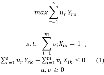
(Charnes, et al., 1978) proposed a technique to aggregating the outptus in a virtual outputs and the inputs in a virtual inputs and use the ratio virtual output/virtual input to represent the relative efficiency of a production units (named Decision Making Units- DMU). In its dual formulation the technique envelop the observations by production function. The technique was named Data Envelopment Analysis (DEA). Since the functional form need not be specificated it is a non parametric approach. So, to measure the performance applying the multiplier formulation of the model we obtain the following linearized input program (after Charnes transformation):
𝑚𝑎𝑥 ∑ 𝑢
𝑟𝑠
𝑟=1
𝑌
𝑟𝑜𝑠. 𝑡. ∑ 𝑣𝑖𝑋𝑖𝑜
= 1
𝑚𝑖=1
,
∑
𝑠𝑟=1𝑢
𝑟𝑌
𝑟𝑘− ∑
𝑚𝑖=1𝑣
𝑖𝑋
𝑖𝑘≤ 0
(1)
𝑢, 𝑣 ≥ 0
Once solved the program (1) the optimal solution 𝑢∗, 𝑣∗ are obtained. So, the efficiency will be:
∑ 𝑢𝑟∗𝑌𝑟𝑜 𝑠
𝑟=1
[image:6.595.216.395.375.505.2]The model above is a DEA “black box” model which is graphically showed in the Figure 2 below.
In the following subsection we will show the NDEA models and two techniques to conduct the relative efficency measurement for the systems (organization/producion process) and its parts (divisions/stages) displayed in the Figure 1 above.
3.2 The NDEA models formulation
In this section we formulate a relational NDEA model to calculate the efficiency of the process in Figure 1. The efficiency measurement of its subprocess will be showed in the subsection (3.3) where we will use two ways to do this, one of this, according our knowledge, we believe to be new and never adopted. Assuming Constant Return to Scale (CRS) the corresponding input oriented multiplier relational NDEA model for the process displayed in the Figure 1 above[ (Kao, 2017)]7 will be:
max 𝑣1𝑌3+ 𝑣2𝑌4+ 𝑣3𝑌5
𝑠. 𝑡. 𝑢1𝑋1+ 𝑢2𝑋2+ 𝑢3𝑋3+ 𝑢4𝑋4+ 𝑢5𝑋5= 1
(𝑤1𝑌1+ 𝑤2𝑌2) − (𝑢1𝑋11+ 𝑢2(1 − 𝛼1− 𝛽1)𝑋21+ 𝑢3(1 − 𝛼2− 𝛽2)𝑋31) ≤ 0 𝐼 𝑠𝑢𝑏 ( model 1)
(𝑣1𝛿1𝑌3(2)+ 𝑣2𝛿2𝑌4(2)+ 𝑣3𝛿3𝑌5(2)) − (𝑤1(1 − 𝛾1)𝑌1(12)+ 𝑤2(1 − 𝛾2)𝑌2(12)+ 𝑢4𝑋4+ 𝑢2𝛼1𝑋2(2)+ 𝑢3𝛼2𝑋3(2)) ≤ 0 𝐼𝐼 𝑠𝑢𝑏
(𝑣1(1 − 𝛿1)𝑌3(3)+ 𝑣2(1 − 𝛿2)𝑌4(3)+ 𝑣3(1 − 𝛿3)𝑌5(3)) − (𝑢2𝛽1𝑋2(3)+ 𝑢3𝛽2𝑋3(3)+ 𝑢5𝑋5+ 𝑤1𝜋1𝑌1(13)+ 𝑤2𝜋2𝑌2(13)) ≤ 0 𝐼𝐼𝐼 𝑠𝑢𝑏 (𝑣1𝑌1+ 𝑣2𝑌2+ 𝑣3𝑌3) − (𝑢1𝑋1+ 𝑢2𝑋2+ 𝑢3𝑋3+ 𝑢4𝑋4+ 𝑢5𝑋5) ≤ 0 𝑠𝑦𝑠𝑡𝑒𝑚
Where:
X1,X2,X3,X4,X5= system resources
Y3 , Y4, Y5= outputs system
X1(1),X2(1),X3(1)= resources I sub-process
Y1,Y2= outputs I sub- process
Y1(12),Y2(12)= relational resources between the I and the II sub-process
Y1(13),Y2(13)= relational resources between the I and the III sub-process
X2(2),X3(2)=shared inputs resources between the I and the II sub-process
X4=exogenous resources II sub-process
Y3(2),Y4(2),Y5(2)= outputs II sub-process
X5= resources III sub-process
X2(3),X3(3),= shared resources between I and III sub-process
Y1(13),Y2(13)= shared outputs resources between I and III sub-process
7
Y3 (3)
,Y4 (3)
,Y5 (3)
= outputs third sub-process
α1, α2= proportion of the shared inputs varibles X22, X32 respectively
β1, β2= proportion of the shared inputs variables X23, X33 respectively
γ1, γ2= proportion of the shared intermediate variables Y1(12), Y2(12) respectively and
π1, π2= proportion of shared intermediate variables between the I and III subprocess Y1(13), Y2(13) respectively
δ1, δ2, δ3= proportion of the shared outputs variables Y3(2), Y4(2), Y5(2) and (1 − 𝛅) the proportion of , Y3(3), Y4(3), Y5(3)
With this formulation the same inputs and outputs will receive the same weights [ (Kao, 2009(a))]. The operation of each process is descripted with the constraints in the model 1. For example the constraints sub1 indicate the operations of the first subprocess. The constraint sub 2 consider the operations of the second subprocess, and so on. The relational nature of the model 1 is that the outputs of the first subprocess (𝑌1, 𝑌2) receive the same weights (𝑤1, 𝑤2) of the relational variables that connect it with the second subprocess
(𝑌1(12), 𝑌2(12)) and third subprocess (𝑌1(13), 𝑌2(13)). So, as stated in others parts in the paper the same variables (in this case 𝑌1 𝑎𝑛𝑑 𝑌2) receive the same weights. The proportion assigned to the variables of each subprocess can be differently defined [ (Kao, 2017)]. Here we assigned a fixed proportion (i.e. 𝛼1, 𝛼2 for the variables 𝑋22, 𝑋32) without any specific intention. This latter step (the asssignement of the proportions) is of crucial interest for the purposes of policy indications.
3.3 The efficiency measurement: two approaches
According to the relational network approach [ (Kao, 2009(a))] once solved the model 1 above the efficiency of the system (Esys ) is given by :
𝐸𝑠𝑦𝑠= 𝑣1∗𝑌3+𝑣2∗𝑌4+𝑣3∗𝑌5
𝑢1∗𝑋1+𝑢2∗𝑋2+𝑢3∗𝑋3+𝑢4∗𝑋4+𝑢5∗𝑋5= 𝑣1
∗𝑌
3+ 𝑣2∗𝑌4+ 𝑣3∗𝑌5 (formula 1)
Meanwhile the efficiency of the subprocess will be produced by its contraints as follow:
𝐸𝐼= 𝑤1∗𝑌1+𝑤2∗𝑌2
𝑢1∗𝑋
11+𝑢2∗(1−𝛼1−𝛽1)𝑋21+𝑢3∗(1−𝛼2−𝛽2)𝑋31 (formula 2)
𝐸𝐼𝐼= 𝑣1∗𝛿1𝑌3(2)+𝑣2∗𝛿2𝑌4(2)+𝑣3∗𝛿3𝑌5(2)
𝑢4𝑋4+𝑤1𝛾1𝑌1(12)+𝑤2𝛾2𝑌2(12)+𝑢2𝛼1𝑋22+𝑢3𝛼2𝑋32 (formula 3)
𝐸𝐼𝐼𝐼 = 𝑣1∗(1−𝛿1)𝑌3(3)+𝑣2∗(1−𝛿2)𝑌4(3)+𝑣3∗(1−𝛿3)𝑌5(3)
𝑢5∗𝑋5+𝑢3∗𝛽2𝑋3(3)+𝑢2∗𝛽1𝑋2(3)+𝑤2∗𝜋2𝑌2(13)+𝑤1∗𝜋1𝑌1(13)
(formula 4)
Figure 3 System with block
The Block 1 internally is a well structured system [according to (Kao, 2009(a));(Kao, 2014)], in particular would be a series configuration with shared inputs variables [ (Kao, 2017)]. To build this block we assumed that relatively to the original system model ( see Figure 1) it possible to assign to each sub-process/block own indipendent resources eliminating the link between them (in particular the inputs sharing condition with the stage 3). In this case the approach proposed here conducted to modeling the original system with a block (block 1) and a stage with sharing outputs. This strategy would avoid the introduction of the dummy subprocess in the case of unstructured model with three stages. This solution, according our opinion, can improve the interpretation and the measurement of the efficiency of the system and its subparts. In fact once introduced the block 1 in our trasformation will have that the efficiency of the block 1 will be calculated as a structured series network model, and the efficiency of the third subprocess, without shared outputs with the block 1,will be calculated as an indipendend DEA model once assigned to it the proportion of output produced. This strategy beyond to the ease efficiency measurement is of interest to managerial or policy objectives. For example, can happen, that inside a system two subsytems cannot be separate for technical motivation or others motivations. As can happen in the case of hospital ordinary acute care (Harris, (Autumn,1977)). Where don’t have sense to consider assistance activity without medical activity for acute ordinary inpatient and hospital medical care whitout followed to the assistance activity. While may be of interest, by organization or policy point of view, to keep the rehabilitation services separate from the rest of the hospital services. A characteristic of our proposal is based on the possibilities to consider the variables of the subsystem as indipendent. In other words, for example, instead to consider the beds as shared variables, as happen in the relational model, we consider the beds of the first and the third subprocess as differents inputs. The immediate implication of this, relatively to the relational model, is that beds and medical staff variables of the production process treated here will receive in the transformed system (Figure 2) differents weights. So, the correspondig efficiency measurement will require to solve first the following relational NDEA model for the Block 1:
max 𝑣1𝛼𝑌1
𝑠. 𝑡. 𝑢1𝑋1 + 𝑢2𝑋2 + 𝑢3𝑋3 + 𝑢4𝑋4 = 1 (model 2 ) (𝑤1𝑍12 + 𝑤2𝑍22) − (𝑢1𝑋1 + 𝑢2𝜎1𝑋2 + 𝑢3𝜎2𝑋3 + 𝑢4𝑋4) ≤ 0
𝑣𝛼𝑌1 − (𝑤1𝑍12 + 𝑤2𝑍22 + 𝑢2(1 − 𝜎1)𝑋2 + 𝑢3(1 − 𝜎2)𝑋3 − 𝑢4𝑋4) ≤ 0
𝑣1𝑌1 − (𝑢1𝑋1 + 𝑢2𝑋2 + 𝑢3𝑋3 + 𝑢4𝑋4) ≤ 0
Where 𝜎1, 𝜎2 are the proportions of the variables 𝑋2 𝑎𝑛𝑑 𝑋3 respectively assigned to the first subprocess and
(1 − 𝜎1)𝑎𝑛𝑑 (1 − 𝜎2)the proportions of the same variables assigned to the second subprocess. 𝛼 is the
𝐸𝐵𝑙𝑜𝑐𝑘1= 𝑣1∗𝛼𝑌1
(𝑢1∗𝑋1+𝑢 2 ∗𝑋2+𝑢
3 ∗𝑋3+𝑢
4
∗𝑋4)= 𝑣1∗𝛼𝑌1 (formula 5)
Later we will solve the following standard DEA model for the remaining subprocess (here the subprocess 3):
………
max 𝑣2𝛽𝑌2
𝑠. 𝑡. 𝑢5𝑋5+ 𝑢6𝑋6+ 𝑢7𝑋7+ 𝑢8𝑋8+ 𝑢9𝑋9= 1 (model 3) 𝑣2𝛽𝑌2 − (𝑢5𝑋5+ 𝑢6𝑋6+ 𝑢7𝑋7+ 𝑢8𝑋8+ 𝑢9𝑋9) ≤ 0
To the model 3 we will obtain the following optimal values: 𝑣2∗, 𝑢5∗, 𝑢6∗, 𝑢7∗, 𝑢8∗, 𝑢9∗. So, the efficiency of the third subprocess will be:
𝐸𝐼𝐼𝐼= 𝑣2∗𝛽𝑌2
𝑢5∗𝑋5+𝑢6∗𝑋6+𝑢7∗𝑋7+𝑢8∗𝑋8+𝑢9∗𝑋9= 𝑣2
∗𝛽𝑌2 (formula 6)
The efficiency of the whole subprocess can be calculate using the weighted additive efficiency decomposition [ (Chen, et al., 2009b)] as follow:
𝐸𝑠𝑦𝑠𝑏𝑙𝑜𝑐𝑘= 𝜏1𝐸𝑏𝑙𝑜𝑐𝑘+ 𝜏2𝐸𝐼𝐼𝐼 (formula 7)
Where 𝜏1≥ 0, 𝜏2≥ 0 with 𝜏1+ 𝜏2= 1, reflect the importance of the suprocess/block in the efficiency measurement. This latter approach, that used the blocks trasformation is different to the relational approach to the fact that, the variable of the subprocess and the variables of block 1 are treated as not relational variables. In fact, as stated above, we have differents weights for each inputs subprocess variables So, for example the variable X2 and X5 can represent the same resouce (i.e. beds in this example) but are treated as different variables with own weights. This can be of same utility in some situations where for some parts of the whole subprocess exist technological, organizational or/and legislative contraints .
4. The application to the hospitals
The efficiency measurement in the health care/hospitals setting when its internal structure is considered is relatively recent.[i.e. (Chilingerian, et al., 2004); (Kawaguchi, et al., 2014); (Pinto, 2016)]. Chilingerian et al. 2004 consider a two stage process in measuring the phisicians care and apply two separate DEA. The first stage has as inputs registererd nurses, medical supplies, and capital and fixed costs. These inputs generate the outputs as patient days, quality of treatment, drugs dispensed, among others. These first stage outptus are the inputs of the second stage to generate as outptus research grants, quality patients, and quantity of individual trained, by speciality. Kawaguchi et al 2014 evaluate the policy effects of the health reform in Japan on the hospital efficiency considering this latter as organizations with two internal heterogenous organizations. In particular the authors apply the dynamic-network data envelopment analysis. Pinto 2016 consider a two stage process in the hospitals acute care applying the network DEA approach to estimates the relative efficiency of it. In Pinto,2016 the second stage has an exogenous inputs confering the non linearity to the model.In this paper we proposed in the subsection 3.2,acording our opinion, a new approach in the case of a three stages process. In this section we apply it to the hospital acute care services addying a third process at the process in (Pinto, 2016). The variables used here are the same in (Pinto, 2016) (see Table 1)
Table 1. Hospital acute care’s production process variables
Inputs Outputs Relational variables
Physicians Ordinary discharges Surgical interventions
Ordinary beds Day-hospital discharges Days-on hospitals
Day-hospital beds Surgical discharges Shared resources
Day-surgery beds
Nurses (second sub-process)
Medical-technical staff (not included)
Rehabilitative staff
The role of the some variables inside the relational model will depend to how the production process will be modeled. Here, the variables of the relational NDEA model in the case of hospitals acute care production process with three stages as in the Figure 1 above will be:
X1,X2,X3,X4,X5= system resources: physicians, nurses, beds, rehabilitative staff, medical-technical-staff
Y3 , Y4, Y5= outputs system:ordinary discharges, day-hospital discharges, surgical discharges, respectively
X1(1),X2(1),X3(1)= resources of the I sub-process:physicians, beds, medical-technical-staff, respectively
Y1,Y2= outputs of the I sub- process :surgical interventions, days on hospitals, respectively
Y1 (12)
,Y2 (12)
= relational resources between the I and the II sub-process:surgical interventions, days on hospitals, respectively
Y1(13),Y2(13)= relational resources between the I and the III sub-process:surgical interventions, days on hospitals,
respectively
X2(2),X3(2)=shared inputs resources between the I and the II sub-process (beds, medical-technical-staff)
X4=exogenous resources of the II sub-process:nurses, respectively
Y3(2),Y4(2),Y5(2)= outputs of the II sub-process: ordinary discharges, day-hospital discharges,surgical discharges,
respectively
X5= resources of the III sub-process: rehabilitative staff , respectively
X2(3),X3(3),= shared resources between I and III sub-process: beds, medical-technical-staff , respectively
Y1(13),Y2(13)= shared outputs resources between I and III sub-process: surgical interventions, patients days, respectively
Y3(3),Y4(3),Y5(3)= outputs of the third sub-process:ordinary discharges, day-hospital discharges, surgical discharges,
respectively
𝛼1,𝛼2=proportion of the shared inputs variables X2(2),X3(2) respectively
𝛽1, 𝛽2=proportion of the shared inputs variables X2(3),X3(3) respectively
𝛾1, 𝛾2= proportion of the shared intermediate variables Y1(12),Y2(12) respectively and
𝜋1, 𝜋2= proportion of shared intermediate variables between the I and III subprocess Y1(13),Y2(13) respectively
𝛿1, 𝛿2. 𝛿3=proportion of the shared outputs variables Y3 (2)
,Y4 (2)
,Y5
(2) and (1-δ) the proportion of ,Y 3
(3)
,Y4 (3)
,Y5 (3)
using data on these variables we will have the following optimal weights (additional file1 .xlsx ) and the followinw relative efficiencies (see Table 2 below for its descriptive statistics).
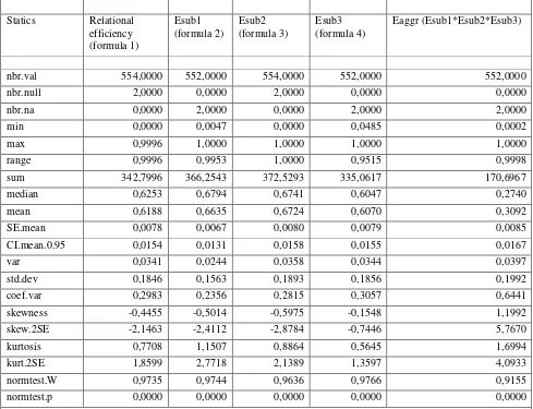
Table 2 Descriptive statistics of NDEA relational efficiency and its subprocess
Statics Relational efficiency (formula 1)
Esub1 (formula 2)
Esub2 (formula 3)
Esub3 (formula 4)
Eaggr (Esub1*Esub2*Esub3)
nbr.val 554,0000 552,0000 554,0000 552,0000 552,0000
nbr.null 2,0000 0,0000 2,0000 0,0000 0,0000
nbr.na 0,0000 2,0000 0,0000 2,0000 2,0000
min 0,0000 0,0047 0,0000 0,0485 0,0002
max 0,9996 1,0000 1,0000 1,0000 1,0000
range 0,9996 0,9953 1,0000 0,9515 0,9998
sum 342,7996 366,2543 372,5293 335,0617 170,6967
median 0,6253 0,6794 0,6741 0,6047 0,2740
mean 0,6188 0,6635 0,6724 0,6070 0,3092
SE.mean 0,0078 0,0067 0,0080 0,0079 0,0085
CI.mean.0.95 0,0154 0,0131 0,0158 0,0155 0,0167
var 0,0341 0,0244 0,0358 0,0344 0,0397
std.dev 0,1846 0,1563 0,1893 0,1856 0,1992
coef.var 0,2983 0,2356 0,2815 0,3057 0,6441
skewness -0,4455 -0,5014 -0,5975 -0,1548 1,1992
skew.2SE -2,1463 -2,4112 -2,8784 -0,7446 5,7670
kurtosis 0,7708 1,1507 0,8864 0,5645 1,6994
kurt.2SE 1,8599 2,7718 2,1389 1,3597 4,0933
normtest.W 0,9735 0,9744 0,9636 0,9766 0,9155
normtest.p 0,0000 0,0000 0,0000 0,0000 0,0000
Legend: ndr.var:number of observations; nrr.null: number of null values; nbr.na:number of missing value; min;max;range;sum: sum of all non-missing values ;media;mean;SE.mean:standard error on the mean ; CI.mean.:the confidence interval of the mean at the p level; var:; stad.var;coef.var:variation coefficient defined as the standard deviation divided by the mean ;skewness:skewness coefficient ;skew.2SE:its significant criterium ( if skew.2SE > 1, then skewness is significantly different than zero), ;kurtosis:kurtosis coefficient ;kurt.2SE:its significant criterium;normtest.W:statistic of a Shapiro-Wilk test of normality ;normtest.p:its associated probability .
Instead, adopting the other model above (model 2) we will have the following variables:
X1,X2,X3,X4= block 1 resources: physicians, beds,, medical-technical-staff, nurses, respectively Y1= block 1 outputs:ordinary discharges, day-hospital discharges, surgical discharges, respectively Z11,Z22= intermediate varibels block 1: surgical interventions, days on hospitals, , respectively X22,X32= block 1shared resources:beds,, medical-technical-staff, respectively
Solving the model 2and 3 and appliyng the formulas 5,6,7 we will have the following efficiencies scores (see Table 2) and optimal weights (additional file2 and 3 .xlsx):
Statistics Esysblock1 (formula 7)
Esysblock1a (formuma 7)
Esysblock1b (formula 7)
Eblock1 (formula 5)
effstage3 (formula 6)
nbr.val 554,0000 554,0000 554,0000 554,0000 554,0000
nbr.null 2,0000 2,0000 2,0000 2,0000 2,0000
nbr.na 0,0000 0,0000 0,0000 0,0000 0,0000
min 0,0000 0,0000 0,0000 0,0000 0,0000
max 1,0000 1,0000 1,0000 1,0000 1,0000
range 1,0000 1,0000 1,0000 1,0000 1,0000
sum 371,5069 372,2177 369,3743 368,6634 375,7720
median 0,6757 0,6749 0,6720 0,6700 0,6821
mean 0,6706 0,6719 0,6667 0,6655 0,6783
SE.mean 0,0085 0,0085 0,0085 0,0085 0,0088
CI.mean.0.95 0,0167 0,0167 0,0167 0,0167 0,0174
var 0,0399 0,0401 0,0399 0,0401 0,0433
std.dev 0,1997 0,2003 0,1997 0,2004 0,2081
coef.var 0,2978 0,2982 0,2996 0,3011 0,3068
skewness -0,5775 -0,5760 -0,5532 -0,5336 -0,5319
skew.2SE -2,7823 -2,7749 -2,6653 -2,5704 -2,5626
kurtosis 0,6047 0,5757 0,6106 0,5927 0,3847
kurt.2SE 1,4593 1,3893 1,4733 1,4302 0,9284
normtest.W 0,9642 0,9644 0,9648 0,9648 0,9602
normtest.p 0,0000 0,0000 0,0000 0,0000 0,0000
In the Table 2 the additive efficiency aggregation (formula 7) it has been calculate using different values of
𝜏. In particular : Esysblock1 consider 𝜏1= 0.6, 𝜏2= 0.4, Esysblock1a 𝜏1= 0.5, 𝜏2= 0.5 and Esysblock1b
𝜏1= 0.9, 𝜏2= 0.1. To compare the efficiencies of the two models (model 1 relational NDEA, and model 2
network system with block) we plot the empirical cumulative distribution functions (see Figure 4),also.
Figure 4 Empirical cumulative distribution of efficiency scores model 1 and 2
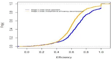
At the same way we compare the efficiecies of the subprocess 3 (see Figure 5).
The blue curve is the empirical cumulative distribution function of the efficiency score of the third stage calculate with a DEA standard model in line with the block approach above (formula 6). Meanwhile the orange curve is the efficiency of the subprocess three calculate using the multiplicative decomposition apparoach in the relational NDEA model (formula 4). As we can note the two functions are very different from each other. This is the effect of differents optimal weights for the same variables. In other words for example the optimal weight for the medical technical staff in the relational model is always the same, whether we consider the first subprocess that the third. In the case of block approach despite the fact the third subprocess became indipendent to the input poit of view to the firs subprocess th eoptimal weight fot the varible medical-technical staff differ according to which we consider the first or third subprocess . Despite the fact the optimal weights in this approach (DEA and NDEA) has evident policy values [ (Smith, et al., 2005)], the two approach produce different policy considerations in general and for the third subprocess here. An useful thing is to calculate the descriptive statistics of all the efficiency scores of the third subprocess (see Table 4)
Table 4 Efficiency scores of the third subprocess under model1 and model 2
Statistics effstage3 (formula 6 ) Esub3 (formula 4)
nbr.val 554,0000 552,0000
nbr.null 2,0000 0,0000
nbr.na 0,0000 2,0000
min 0,0000 0,0485
max 1,0000 1,0000
range 1,0000 0,9515
sum 375,7720 335,0617
median 0,6821 0,6047
mean 0,6783 0,6070
SE.mean 0,0088 0,0079
CI.mean.0.95 0,0174 0,0155
var 0,0433 0,0344
std.dev 0,2081 0,1856
coef.var 0,3068 0,3057
skewness -0,5319 -0,1548
skew.2SE -2,5626 -0,7446
kurtosis 0,3847 0,5645
kurt.2SE 0,9284 1,3597
[image:14.595.198.385.85.183.2]normtest.p 0,0000 0,0000
[image:15.595.52.541.233.586.2]Although the Table 4 outline a little difference in the mean of the two process their distribution is significantly different as we can see in the Figure 4. In fact the efficiency scores empirical distribution function of the third stage calculated under the multiplicative efficiency decomposition is more concave than the those calculate in the case of block approach (subsection 3.2). The DEA efficiency score (1) are in Table 5 below.
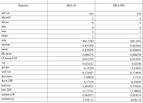
Table 5 DEA efficiency score: the black box performance measurement
Statistics DEA-D DEA-ND
nbr.val 554 554
nbr.null 2 2
nbr.na 0 0
min 0 0
max 1 1
range 1 1
sum 464,7384 469,1283
median 0,857498 0,865461
mean 0,838878 0,846802
SE.mean 0,006275 0,006296
CI.mean.0.95 0,012325 0,012367
var 0,021812 0,02196
std.dev 0,14769 0,14819
coef.var 0,176057 0,174999
skewness -1,69626 -1,7123
skew.2SE -8,17169 -8,24899
kurtosis 5,692925 5,578384
kurt.2SE 13,73721 13,46082
normtest.W 0,864577 0,855679
normtest.p 1,77E-21 4,02E-22
The column D refer to the DEA score efficiency with all discretional inputs, while the column DEA-ND refer DEA efficiency scores in the case of not discretional inputs. In this case we posed the variables nurse as not discretional as example. The effecct of the non discretionality assumption, in terms of performance management, can be observed on the values of the descriptive statistic in the Table 5 above and in the histogram and empirical cumulative distributoin function of the DEA efficiency score in the Figure 6 below.
5. Discussion and conclusions
The economic modeling of a production process is very often conduct using the production function approach, meanwhile the use of econometric model allow to measure its efficiency as happen for example in the case of SFA [ (Battese, et al., 1977)]. In others cases the estimation of the production function and consequent measurement of the efficiency of production process is conduct using models mathematically founded as happen in the case of DEA [ (Cooper, et al., 2007); (Cooper, et al., 2007)]. All these ways to modeling and measure the efficiency of a production process do not allow to think to the production process as a system composed of different part linked among them. Not a long time ago, some author introduced the idea to modeling the produciton process as a system of part interconnected [ (Fa¨re, et al., 1996a); (Fa¨re, et al., 1996b)] and later great progress are made in this direction as happend in [ (Kao, 2014); (Kao, 2009(a)); (Kao, 2017)] that introduced two basic models: a series model and a parallel model. Here, we modeled a production process as a system of three subprocess/stages interconnected among them (see Figure.1). This model it has been applied to the hospital acute care production services overcoming the conceptualization in (Pinto, 2016). Differently to (Pinto, 2016) the hospital acute care production process proposed here consider in addition to the medical and assistance activity the rehabilitaive activity as an acute hospital of treatment activities. This offered us the opportunities to modeling a process with three stages using the relational NDEA model to measure its efficiency. However, in addition to the multiplicative efficiency decompostion we propose an approach with blocks. In this later case we not apply the relational NDEA approache to etimates the relative efficiency. Generating with our approach, according our opinion, evidents and useful policy implications. The model (model 1) is characterized by intermediate flows (network strucure), shared variables (shared model) and exogenous variables for one of the subprocess. One variant, here not considered, can use exogenous variables for the whole process to gave multi-stage nature at the model [ (Kao, 2017)]. The efficiency of the relational model it has been calculate via program 1. Instead, the efficiency of its parties are obtained following two ways. The first is the multiplicative decomposition efficiency, according to, once obtained the optimal weights to the program 1 the weightes are applied to calculate the efficiency of the three stages following the formulas 1,2,3,4. The second way proposed consist in to isolate inside the process a block (subsection 3.3). This approach it has been proposed, according our opinion, to improve the interpretation of the efficiency results when the internal structure of a unstructured system is considered. In fact, in this latter approach the efficiency of the system will be obtained using the weights additive efficiency aggregation. In this way it is possible assign to the block a weight that reflect the importance of it inside the process. The block approach can be useful in the case of policy objectives, also. The paper showed the application of the model in the case of the hospitals services. In this latter case the
“block” strategy appear very useful, despite the fact often is convenient treating two sub-part togheter. The
modeling the internal structure of the hospital acute care production process whit three subprocess, the second, that can be allocated inside the efficiency measurement in the case of general DEA literaure in the case of network structure cosideration, consist in the proposal of the “block” approach to think again the original process in key of policy indications. In fact these latter can suggest to consider two or more stages inside a production process as an unique block, as in the text stated.
References
Aigner, D.J., Lovell, C.A.K. e Schmidt, P. 1977. Formulation and estimation of stochastic frontier production functions. Journal of Econometrics. 1977, Vol. 6, p. 21–37.
Baker, K.R. e Kropp, D.H. 1985. Management Science: An Introduction to the Use of Decision Models. New York : Wiley, 1985.
Battese, G.E. e Corra, G.S. 1977. ESTIMATION OF A PRODUCTION FRONTIER MODEL: WITH
APPLICATION TO THE PASTORAL ZONE OF EASTERN AUSTRALIA. Australian Journal of
Agricultural and Resource Economics. 1977, Vol. 21, 3.
Castelli, L. e Pesenti, R. 2014. Network, Shared Flow and Multi-level DEA Models: A Critical Review. [aut. libro] W.D. Cook and J. Zhu. Data Envelopment Analysis, International Series in Operations Research & Management Science. New York : Springer Science+Business Media, 2014, Vol. 208, 15, p. 329-366. Castelli, L., Pesenti, R. e & Ukovich, W. 2004. DEA-like models for the efficiency evaluation of hierarchically structured units. European Journal of Operational Research. 2004, Vol. 154, 2, p. 465-476. Castelli, L., Pesenti, R. e Ukovich, W. 2010. A classification of DEA models when the internal structure of the Decision Making Units is considered. Annals of Operations Research. 2010, Vol. 173, p. 207–235. Castelli, L., Pesenti, R. e Ukovicha, W. 2001. DEA-like models for efficiency evaluations of specialized and interdependent units. European Journal of Operational Research. 2001, Vol. 132, 2, p. 274-286.
Charnes, A., Cooper, W. W. e Rhodes, E. 1978. Measuring the efficiency of decision making units.
European Journal of Operational Research. 1978, Vol. 2, p. 429-444.
Chen, Y. e Zhu, J. 2004. Measuring information technology’s indirect impact on firm peformance.
Information Technology & Management Journal. 2004, Vol. 5, 1-2, p. 9-22.
Chen, Y., et al. 2009b. Additive efficiency decomposition in two-stage DEA. European Journal of Operational Research. 2009b, Vol. 196, p. 1170-1176.
Chen, Y., et al. 2010 b. DEA model with shared resources and efficiency decomposition. European Journal of Operational Research. 2010 b, Vol. 207, p. 339–349.
Chilingerian, J. e Sherman, H. D. 2004. Health care applications: From Hospitals to Physician, from productive efficiency to quality frontiers. [aut. libro] L. M. Seiford, & J. Zhu W. W. Cooper. Handbook on data envelopment analys. Boston : Springer, 2004.
Coelli, T.J., et al. 2005. An Introduction to Efficiency and Productivity Analysis. 2nd Edition. s.l. : Springer, 2005. ISBN 978-0-387-24266-8.
Cook, W.D. e Seiford, L.M. 2009. Data envelopment analysis (DEA)—thirty years on. European Journal of Operational Research. 2009, Vol. European JournalofOperationalResearch2009;192:1–17., p. 1–17.
Cooper, W. W., Seiford, Lawrence M. and Tone, K. 2007. Data Envelopment Analysis. A Comprehensive Text with Models, Application, References and DEA-Solver Software. New York : Springer, 2007.
Cooper, W.W., Seiford, L.M. e ToneK, Zhu J. 2007. Some models and measures fo revaluating performances with DEA:past accomplishments and future prospects. Journal of Productivity Analysis . 2007, Vol. 28, p. 151–163.
Daraio, C. e Simar, L. 2008. Advanced Robust and Nonparametric Methods in Efficiency Analysis. Methodology and Applications. s.l. : Springer, 2008.
Deprins, D., Simar, L. e Tulkens, H. 1984. Measuring Labor-Efficiency in Post Office. [aut. libro] M in Marchand, P. Pestieu e H. Tulkens. The performance of Public Interprises: Concepts and Measurement.
Amsterdam : s.n., 1984, p. 243-267.
Fa¨re, R. e & Grosskopf, S. 1996a. Intertemporal production frontiers: with dynamic DEA. Boston : Kluwer, 1996a.
Fa¨re, R. e Grosskopf, S. 1996b. Productivity and intermediate products:A frontier approach. Economics Letters. 1996b, Vol. 50, p. 65-70.
Fa¨re, R. e Whittaker, G. 1995. An intermediate input model of dairy production using complex survey data.
J Agric Econ. 1995, Vol. 46, p. 201-213.
Greene, W.H. 1980. Maximum likelihood estimation of econometric frontier functions. J. Econometrics.
1980, Vol. 13:, p. 27 -56.
Harris, J.E. (Autumn,1977). The Internal Organization of Hospitals: Some Economic Implications. The Bell Journal of Economics. (Autumn,1977), Vol. 8, 2, p. 467-482.
Hiller, F.S. e Lieberman, G.J. 2001. Introduction to Operation Research. s.l. : McGraw-Hill Series in Industrial Engineering and Management Science, 2001. ISBN 0-07-232169-5 .
Kao, C. e Hwang, S-N. 2008. Efficiency decomposition in two-stage data envelopment analysis: An application to non-life insurance companies in Taiwan. European Journal of Operational Research. 2008, Vol. 185, 418-429.
Kao, C. 2014. Efficiency decomposition for general multi-stage systems in data envelopment analysis.
European Journal of Operational Research. 2014, Vol. 232, p. 117-124.
—. 2009(a). Efficiency decomposition in network data envelopment analysis: A relational model. European Journal of Operational Research. 2009(a), Vol. 192, 949-962.
—. 2017. Network Data Envelopment Analysis. Foundation and Extension. s.l. : Springer, 2017. Vol. 240. ISBN 978-3-319-31718-2.
Kawaguchi, H, Tone, K. e Tsutsui, M. 2014. Estimation of the efficiency of Japanese hospitals using dynamic and network Data envelopment Analysis model. Health Care Management Sciences. 2014, Vol. 17, p. 101-112.
Li, Y., Chen, Y.,Liang,L. e Xie, J. 2012. DEA models for extended two-stage network structures. Omega.
2012, Vol. 40, p. 611–618.
Liang, L., Cook, W. D. e & Zhu, J. 2008. DEA models for two-stage processes: Game approach and efficiency decomposition. Naval Research Logistics. 2008, Vol. 55, p. 643-653.
Liang, L., et al. 2011. DEA Efficiency in two-stage networks with feed back. IIE Transactions. 2011, Vol. 43, p. 309-322.
Liang, L., et al. 2006. DEA models for supply chain efficiency evaluation. Annals of Operations Research.
2006, Vol. 145, 1, p. 35-49.
Liu, J.S., et al. 2013. A survey of DEA applications. Omega. 2013, Vol. 41, p. 893-902.
Meeusen, W. e van den Broeck, J. 1977. Efficiency Estimation from Cobb-Douglas Production Functions with Composed Error. International Economic Review. 1977, Vol. 18, 2, p. 435-44 .
Olesen.O.B. e Petersen, N.C. 2016. Stochastic Data Envelopment Analysis—A review. European Journal of Operational Research. 2016, Vol. 251, 1, p. 2-21.
Ozcan, Y.A. 2008. Health Care Benchmarking and Performance Evaluation. An Assesment using Data Envelopment Analysis (DEA). New York : Springer, 2008. ISBN 978-0-387-75447-5.
Pidd, M. 2003. Tools for Thinking: Modelling in Management Science. Chichester : J. Wiley & Sons Ltd., 2003.
Pinto, C. 2016. The Acute Care Services Production Process’s Efficiency: A DEA Network Model for the Italian Hospitals. Athens Journal of Health. March 2016, Vol. 3, 1.
Premachandra, I. M., et al. 2012. Best-performing US mutual fund families from 1993 to 2008: Evidence from a novel two-stage DEA model forefficiency decomposition. Journal of Banking and Finance. 2012, Vol. 36, 12, p. 3302–3317.
Richmond, J. 1974. Estimating the efficiency of production. Int. Econ. Rev. 1974, Vol. 15: 521., p. 515-521.
Robinson, S. 2008. Conceptual modelling for simulation part I: definition and requirements. Journal of the Operational Research Society. 2008, Vol. 59, 3, p. 278 - 290.
Seiford, L.M. 1996. Data envelopment analysis:the evolution of the state of the art (1978–1995). Journal of Productivity Analysis1996;7:99–137. Journa lof Productivity Analysis. 1996, Vol. 7, p. 99–137.
Sexton, T. e & Lewis, H. 2003. Two–stage DEA: An application to Major League Baseball. Journal of Productivity Analysis. 2003, Vol. 19, 2, p. 227–249.
Smith, P.C. e Street, A. 2005. Measuring the Efficiency of Public Services:The Limits of Analysis. Journal of the Royal Statistical Society. 2005, Vol. 168, 2, p. 401-417.
Thompson, G.E. 1982. Management Science: An Introduction to Modern Quantitative Analysis and Decision Making. . New York : McGraw-Hill Publishing Co, 1982.