Learning attention for historical text normalization by learning to pronounce

Proceedings of the 55th Annual Meeting of the Association for Computational Linguistics, pages 332–344 Vancouver, Canada, July 30 - August 4, 2017. c2017 Association for Computational Linguistics

Proceedings of the 55th Annual Meeting of the Association for Computational Linguistics, pages 332–344 Vancouver, Canada, July 30 - August 4, 2017. c2017 Association for Computational Linguistics

Learning attention for historical text normalization

by learning to pronounce

Marcel Bollmann Department of Linguistics Ruhr-Universität Bochum

Germany

[email protected]

Joachim Bingel Dept. of Computer Science

University of Copenhagen Denmark

[email protected]

Anders Søgaard Dept. of Computer Science

University of Copenhagen Denmark

[email protected]

Abstract

Automated processing of historical texts often relies on pre-normalization to mod-ern word forms. Training encoder-decoder architectures to solve such problems typi-cally requires a lot of training data, which is not available for the named task. We ad-dress this problem by using several novel encoder-decoder architectures, including a multi-task learning (MTL) architecture us-ing a grapheme-to-phoneme dictionary as auxiliary data, pushing the state-of-the-art by an absolute 2% increase in perfor-mance. We analyze the induced models across 44 different texts from Early New High German. Interestingly, we observe that, as previously conjectured, multi-task learning can learn to focus attention during decoding, in ways remarkably similar to recently proposed attention mechanisms. This, we believe, is an important step to-ward understanding how MTL works.

1 Introduction

There is a growing interest in automated process-ing of historical documents, as evidenced by the growing field of digital humanities and the in-creasing number of digitally available collections of historical documents. A common approach to deal with the high amount of variance often found in this type of data is to perform spelling nor-malization (Piotrowski, 2012), which is the map-ping of historical spelling variants to standard-ized/modernized forms (e.g.vnd→und‘and’).

Training data for supervised learning of histor-ical text normalization is typhistor-ically scarce, mak-ing it a challengmak-ing task for neural architec-tures, which typically require large amounts of la-beled data. Nevertheless, we explore framing the

spelling normalization task as a character-based sequence-to-sequence transduction problem, and use encoder–decoder recurrent neural networks (RNNs) to induce our transduction models. This is similar to models that have been proposed for neu-ral machine translation (e.g.,Cho et al.(2014)), so essentially, our approach could also be considered a specific case of character-based neural machine translation.

By basing our model on individual characters as input, we keep the vocabulary size small, which in turn reduces the model’s complexity and the amount of data required to train it effectively. Us-ing an encoder–decoder architecture removes the need for an explicit character alignment between historical and modern wordforms. Furthermore, we explore using an auxiliary task for which data is more readily available, namely grapheme-to-phoneme mapping (word pronunciation), to reg-ularize the induction of the normalization models. We propose several architectures, including multi-task learning architectures taking advantage of the auxiliary data, and evaluate them across 44 small datasets from Early New High German.

Contributions Our contributions are as follows:

• We are, to the best of our knowledge, the first to propose and evaluate encoder-decoder ar-chitectures for historical text normalization.

• We evaluate several such architectures across

44 datasets of Early New High German.

• We show that such architectures benefit from

bidirectional encoding, beam search, and at-tention.

• We also show that MTL with pronuncia-tion as an auxiliary task improves the perfor-mance of architectures without attention.

• We analyze the above architectures and show that the MTL architecture learns attention from the auxiliary task, making the attention mechanism largely redundant.

• We make our implementation publicly

available athttps://bitbucket.org/ mbollmann/acl2017.

In sum, we both push the state-of-the-art in his-torical text normalization and present an analysis that, we believe, brings us a step further in under-standing the benefits of multi-task learning.

2 Datasets

Normalization For the normalization task, we use a total of 44 texts from the Anselm cor-pus (Dipper and Schultz-Balluff, 2013) of Early New High German.1 _{The corpus is a collection of}

manuscripts and prints of the same core text, a reli-gious treatise. Although the texts are semi-parallel and share some vocabulary, they were written in different time periods (between the 14th and 16th century) as well as different dialectal regions, and show quite diverse spelling characteristics. For ex-ample, the modern German word Frau‘woman’ can be spelled as fraw/vraw (Me), frawe (N2), frauwe(St),fraüwe(B2),frow(Stu),vrowe(Ka), vorwe(Sa), orvrouwe(B), among others.2

All texts in the Anselm corpus are manually an-notated with gold-standard normalizations follow-ing guidelines described inKrasselt et al. (2015). For our experiments, we excluded texts from the corpus that are shorter than 4,000 tokens, as well as a few for which annotations were not yet avail-able at the time of writing (mostly Low German and Dutch versions). Nonetheless, the remaining 44 texts are still quite short for machine-learning standards, ranging from about 4,200 to 13,200 to-kens, with an average length of 7,350 tokens.

For all texts, we removed tokens that consisted solely of punctuation characters. We also lower-case all characters, since it helps keep the size of the vocabulary low, and uppercasing of words is usually not very consistent in historical texts. Tok-enization was not an issue for pre-processing these texts, since modern token boundaries have already been marked by the transcribers.

1_{https://www.linguistics.rub.de/} anselm/

2_{We refer to individual texts using the same internal IDs} that are found in the Anselm corpus (cf. the website).

Grapheme-to-phoneme mappings We use learning to pronounce as our auxiliary task. This task consists of learning mappings from sequences of graphemes to the corresponding sequences of phonemes. We use the German part of the CELEX lexical database (Baayen et al., 1995), particu-larly the database of phonetic transcriptions of German wordforms. The database contains a total of 365,530 wordforms with transcriptions in DISC format, which assigns one character to each distinct phonological segment (including affricates and diphthongs). For example, the word Jungfrau‘virgin’ is represented as’jUN-frB.

3 Model 3.1 Base model

We propose several architectures that are ex-tensions of a base neural network architecture, closely following the sequence-to-sequence model proposed bySutskever et al.(2014). It consists of the following:

• an embedding layer that maps one-hot input vectors to dense vectors;

• an encoder RNN that transforms the input se-quence to an intermediate vector of fixed di-mensionality;

• a decoder RNN whose hidden state is initial-ized with the intermediate vector, and which is fed the output prediction of one timestep as the input for the next one; and

• a final dense layer with a softmax activation which takes the decoder’s output and gener-ates a probability distribution over the output classes at each timestep.

For the encoder/decoder RNNs, we use long short-term memory units (LSTM) (Hochreiter and Schmidhuber, 1997). LSTMs are designed to al-low recurrent networks to better learn long-term dependencies, and have proven advantageous to standard RNNs on many tasks. We found no sig-nificant advantage from stacking multiple LSTM layers for our task, so we use the simplest compet-itive model with only a single LSTM unit for both encoder and decoder.

v r o w e (START) f r a u

f r a u (END)

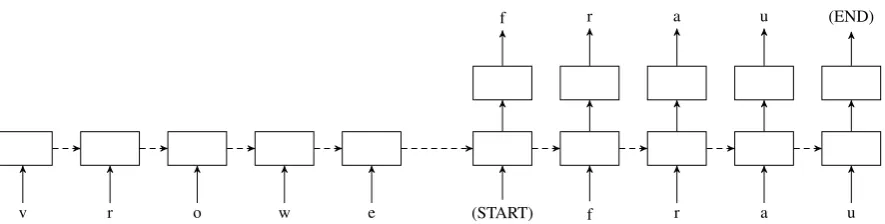
Figure 1: Flow diagram of the base model; left side is the encoder, right side the decoder, the latter of which has an additional prediction layer on top. Multi-task learning variants use two separate prediction layers for main/auxiliary tasks, while sharing the rest of the model. Embedding layers for the inputs are not explicitly shown.

pairs of different lengths. Another important prop-erty is that the model does not start to generate any output until it has seen the full input sequence, which in theory allows it to learn from any part of the input, without being restricted to fixed context windows. An example illustration of the unrolled network is shown in Fig.1.

3.2 Training

During training, the encoder inputs are the histor-ical wordforms, while the decoder inputs corre-spond to the correct modern target wordforms. We then train each model by minimizing the cross-entropy loss across all output characters; i.e., if y = (y1, ..., yn) is the correct output word (as a list of one-hot vectors of output characters) and

ˆ

y = (ˆy1, ...,yˆn) is the model’s output, we mini-mize the mean loss−Pni=1yilog ˆyiover all train-ing samples. For the optimization, we use the Adam algorithm (Kingma and Ba, 2015) with a learning rate of0.003.

To reduce computational complexity, we also set a maximum word length of 14, and filter all training samples where either the input or output word is longer than 14 characters. This only af-fects 172 samples across the whole dataset, and is only done during training. In other words, we evaluate our models across all the test examples.

3.3 Decoding

For prediction, our base model generates output character sequences in a greedy fashion, selecting the character with the highest probability at each timestep. This works fairly well, but the greedy approach can yield suboptimal global picks, in which each individual character is sensibly de-rived from the input, but the overall word is

non-sensical. We therefore also experiment with beam search decoding, setting the beam size to 5.

Finally, we also experiment with using a lexi-cal filter during the decoding step. Here, before picking the next 5 most likely characters during beam search, we remove all characters that would lead to a string not covered by the lexicon. This is again intended to reduce the occurrence of non-sensical outputs. For the lexicon, we use all word forms from CELEX (cf. Sec.2) plus the target word forms from the training set.3

3.4 Attention

In our base architecture, we assume that we can decode from a single vector encoding of the input sequence. This is a strong assumption, especially with long input sequences. Attention mechanisms give us more flexibility. The idea is that instead of encoding the entire input sequence into a fixed-length vector, we allow the decoder to “attend” to different parts of the input character sequence at each time step of the output generation. Impor-tantly, we let the model learn what to attend to based on the input sequence and what it has pro-duced so far.

Our implementation is identical to the decoder with soft attention described byXu et al. (2015). Ifa = (a1, ..., an)is the encoder’s output and ht is the decoder’s hidden state at timestept, we first calculate a context vectorzˆtas a weighted combi-nation of the output vectorsai:

ˆ

zt= n X

i=1

αiai (1)

The weights αi are derived by feeding the en-coder’s output and the deen-coder’s hidden state from the previous timestep into a multilayer perceptron, called the attention model (fatt):

α=sof tmax(fatt(a, ht−1)) (2)

We then modify the decoder by conditioning its internal states not only on the previous hid-den stateht−1 and the previously predicted output characteryt−1, but also on the context vectorzˆt:

it=σ(Wi[ht−1, yt−1,zˆt] +bi) ft=σ(Wf[ht−1, yt−1,zˆt] +bf) ot=σ(Wo[ht−1, yt−1,zˆt] +bo) gt=tanh(Wg[ht−1, yt−1,zˆt] +bg) ct=ftct−1+itgt

ht=ottanh(ct)

(3)

In Eq.3, we follow the traditional LSTM de-scription consisting of input gateit, forget gateft, output gate ot, cell state ct and hidden state ht, whereW andbare trainable parameters.

For all experiments including an attentional de-coder, we use abi-directional encoder, comprised of one LSTM layer that reads the input sequence normally and another LSTM layer that reads it backwards, and attend over the concatenated out-puts of these two layers.

While a precise alignment of input and output sequences is sometimes difficult, most of the time the sequences align in a sequential order, which can be exploited by an attentional component.

3.5 Multi-task learning

Finally, we introduce a variant of the base archi-tecture, with or without beam search, that does multi-task learning (Caruana, 1993). The multi-task architecture only differs from the base archi-tecture in having two classifier functions at the outer layer, one for each of our two tasks. Our aux-iliary task is to predict a sequence of phonemes as the correct pronunciation of an input sequence of graphemes. This choice is motivated by the rela-tionship between phonology and orthography, in particular the observation that spelling variation often stems from phonological variation.

We train our multi-task learning architecture by alternating between the two tasks, sampling one instance of the auxiliary task for each training sample of the main task. We use the encoder-decoder to generate a corresponding output

se-quence, whether a modern word form or a pronun-ciation. Doing so, we suffer a loss with respect to the true output sequence and update the model pa-rameters. The update for a sample from a specific task affects the parameters of corresponding clas-sifier function, as well as all the parameters of the shared hidden layers.

3.6 Hyperparameters

We used a single manuscript (B) for manually evaluating and setting the hyperparameters. This manuscript is left out of the averages reported be-low. We believe that using a single manuscript for development, and using the same hyperparameters acrossallmanuscripts, is more realistic, as we of-ten do not have enough data in historical text nor-malization to reliably tune hyperparameters.

For the final evaluation, we set the size of the embedding and the recurrent LSTM layers to 128, applied a dropout of 0.3 to the input of each recur-rent layer, and trained the model on mini-batches with 50 samples each for a total of 50 epochs (in the multi-task learning setup, mini-batches contain 50 samples of each task, and epochs are counted by the size of the training set for the main task only). All these parameters were set on the B manuscript alone.

3.7 Implementation

We implemented all of the models in Keras ( Chol-let, 2015). Any parameters not explicitly de-scribed here were left at their default values in Keras v1.0.8.

4 Evaluation

We split up each text into three parts, using 1,000 tokens each for a test set and a development set (that is not currently used), and the remainder of the text (between 2,000 and 11,000 tokens) for training. We then train and evaluate on each of the 43 texts (excluding the B text that was used for hyper-parameter tuning) individually.

Avg. Accuracy

Norma 77.89%

Averaged perceptron 75.72%

Bi-LSTM tagger 79.91%

MTL bi-LSTM tagger 79.56%

Base model

GREEDY 78.91%

BEAM 79.27%

BEAM+FILTER 80.46%

BEAM+FILTER+ATTENTION 82.72%

MTL model

GREEDY 80.64%

BEAM 81.13%

BEAM+FILTER 82.76%

BEAM+FILTER+ATTENTION 82.02%

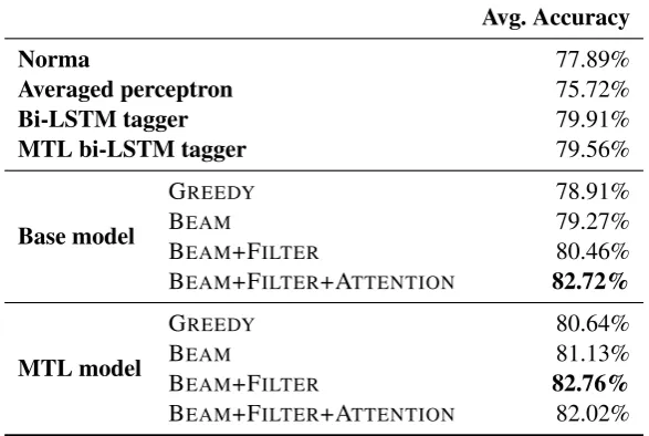
Table 1: Average word accuracy across 43 texts from the Anselm dataset, evaluated on the first 1,000 to-kens of each text. Evaluation on the base encoder-decoder model (Sec.3.1) with greedy search, beam search (k = 5) and/or lexical filtering (Sec.3.3), with attentional decoder (Sec.3.4), and the multi-task

learning (MTL) model using grapheme-to-phoneme mappings (Sec.3.5).

deep bi-LSTM sequential tagger, following Boll-mann and Søgaard (2016). We evaluate this tag-ger using both standard and multi-task learning. Finally, we compare our model to the rule-based and Levenshtein-based algorithms provided by the Norma tool (Bollmann,2012).4

4.1 Word accuracy

We use word-level accuracy as our evaluation metric. While we also measure character-level metrics, minor differences on character level can cause large differences in downstream applica-tions, so we believe that perfectly matching the output sequences is more useful. Average scores across all 43 texts are presented in Table 1 (see AppendixAfor individual scores).

We first see that almost all our encoder-decoder architectures perform significantly better than the four state-of-the-art baselines. All our architec-tures perform better than Norma and the averaged perceptron, and all the MTL architectures outper-formBollmann and Søgaard(2016).

We also see that beam search, filtering, and at-tention lead to cumulative gains in the context of the single-task architecture – with the best archi-tecture outperforming the state-of-the-art by al-most 3% in absolute terms.

For our multi-task architecture, we also observe gains when we add beam search and filtering, but

4_{https://github.com/comphist/norma}

importantly, adding attention does not help. In fact, attention hurts the performance of our multi-task architecture quite significantly. Also note that the multi-task architecture without attention performs on-par with the single-task architecture withattention.

We hypothesize that the reason for this pattern, which is not only observed in the average scores in Table1, but also quite consistent across the indi-vidual results in AppendixA, is that our multi-task learning already learns how to focus attention.

This is the hypothesis that we will try to vali-date in Sec. 5:That multi-task learning can induce strategies for focusing attention comparable to at-tention strategies for recurrent neural networks.

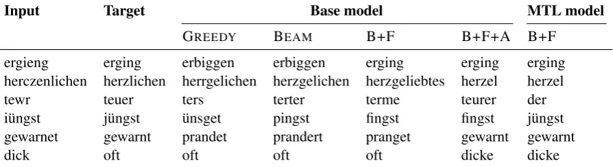
Sample predictions A small selection of pre-dictions from our models is shown in Table 2. They serve to illustrate the effects of the various settings; e.g., the base model with greedy search tends to produce more nonsense words (ters, üns-get) than the others. Using a lexical filter helps the most in this regard: the base model with fil-tering correctly normalizesergiengtoerging‘(he) fared’, while decoding without a filter produces the non-word erbiggen. Even for herczenlichen (modern herzlichen ‘heartfelt’), where no model finds the correct target form, only the model with filtering produces a somewhat reasonable alterna-tive (herzgeliebtes‘heartily loved’).

Input Target Base model MTL model

GREEDY BEAM B+F B+F+A B+F

ergieng erging erbiggen erbiggen erging erging erging

herczenlichen herzlichen herrgelichen herzgelichen herzgeliebtes herzel herzel

tewr teuer ters terter terme teurer der

iüngst jüngst ünsget pingst fingst fingst jüngst

gewarnet gewarnt prandet prandert pranget gewarnt gewarnt

dick oft oft oft oft dicke dicke

Table 2: Selected predictions from some of our models on the M4 text; B = BEAM, F = FILTER, A = AT-TENTION.

only the models with attention or multi-task learn-ing produce the correct normalization, but even when they are wrong, they often agree on the pre-diction (e.g.dicke,herzel). We will investigate this property further in Sec.5.

4.2 Learned vector representations

To gain further insights into our model, we created t-SNE projections (Maaten and Hinton, 2008) of vector representations learned on the M4 text.

Fig.2 shows the learned character embed-dings. In the representations from the base model (Fig.2a), characters that are often normalized to the same target character are indeed grouped closely together: e.g., historical <v> and <u> (and, to a smaller extent,<f>) are often used in-terchangeably in the M4 text. Note the wide sepa-ration of<n>and<m>, which is a feature of M4 that does not hold true for all of the texts, as these do not always display a clear distinction between nasals. On the other hand, the MTL model shows a better generalization of the training data (Fig.2b): here,<u>is grouped closer to other vowel charac-ters and far away from<v>/<f>. Also,<n>and <m>are now in close proximity.

We can also visualize the internal word rep-resentations that are produced by the encoder (Fig.3). Here, we chose words that demonstrate the interchangeable use of<u>and<v>. Histor-icalvnd, vns, vmbbecome modernund, uns, um, changing the<v>to<u>. However, the represen-tation ofvmblearned by the base model is closer to forms likevon, vor, uor, all starting with<v>in the target normalization. In the MTL model, how-ever, these examples are indeed clustered together.

5 Analysis: Multi-task learning helps focus attention

Table1shows that models which employeitheran attention mechanismormulti-task learning obtain similar improvements in word accuracy. However, we observe a decline in word accuracy for models thatcombinemulti-task learning with attention.

A possible interpretation of this counter-intuitive pattern might be that attention and MTL, to some degree, learn similar functions of the in-put data, a conjecture byCaruana(1998). We put this hypothesis to the test by closely investigating properties of the individual models below.

5.1 Model parameters

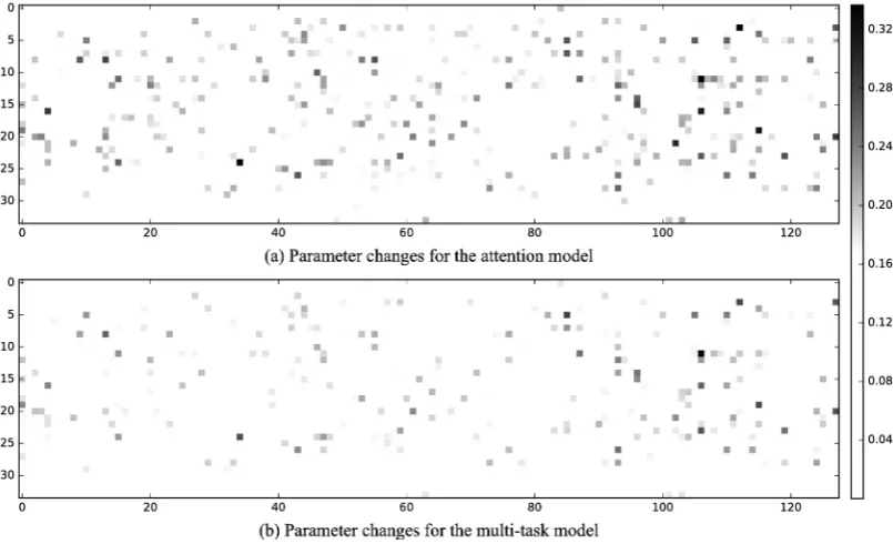
First, we are interested in the weight parameters of the final layer that transforms the decoder output to class probabilities. We consider these parame-ters for our standard encoder-decoder model and compare them to the weights that are learned by the attention and multi-task models, respectively.5

Note that hidden layer parameters are not neces-sarily comparable across models, but with a fixed seed, differences in parameters over a reference modelmaybe (and are, in our case). With a fixed seed, and iterating over data points in the same or-der, it is conceivable the two non-baselines end up in roughly the same alternative local optimum (or at least take comparable routes).

We observe that the weight differences between the standard and the attention model correlate with the differences between the standard and multi-task model by a Pearson’s r of 0.346, averaged across datasets, with a standard deviation of 0.315; on individual datasets, correlation coefficient is as

(a) Base model (b) Multi-task learning model

Figure 2: t-SNE projections (with perplexity 7) of character embeddings from models trained on M4

(a) Base model (b) Multi-task learning model

Figure 3: t-SNE projections (with perplexity 5) of the intermediate vectors produced by the encoder (“historical word embeddings”), from models trained on M4

Figure 5: First-derivative saliency w.r.t. the input sequence, as calculated from the base model (left), the attentional model (center), and the MTL model (right). The scores for the attentional and the multi-task model correlate byρ= 0.615, while the correlation of either one with the base model is|ρ_|<0.12.

high as 96. Figure4illustrates these highly paral-lel weight changes for the different models when trained on the N4 dataset.

5.2 Final output

Next, we compare the effect that employing either an attention mechanism or multi-task learning has on the actual output of our system. We find that out of the 210.9 word errors that the base model pro-duces on average across all test sets (comprising 1,000 tokens each), attention resolves 47.7, while multi-task learning resolves an average of 45.4 er-rors. Crucially, the overlap of errors that are re-solved by both the attention and the MTL model amounts to 27.7 on average.

Attention and multi-task also introduce new er-rors compared to the base model (26.6 and 29.5 per test set, respectively), and again we can ob-serve a relatively high agreement of the models (11.8 word errors are introduced by both models). Finally, the attention and multi-task models dis-play a word-level agreement of κ=0.834 (Co-hen’s kappa), while either of these models is less strongly correlated with the base model (κ=0.817 for attention andκ=0.814 for multi-task learning).

5.3 Saliency analysis

Our last analysis regards the saliency of the input timesteps with respect to the predictions of our models. We follow Li et al. (2016) in calculat-ing first-derivative saliency for given input/output pairs and compare the scores from the differ-ent models. The higher the saliency of an input timestep, the more important it is in determining the model’s prediction at a given output timestep. Therefore, if two models produce similar saliency

matrices for a given input/output pair, they have learned to focus on similar parts of the input dur-ing the prediction. Our hypothesis is that the at-tentional and the multi-task learning model should be more similar in terms of saliency scores than either of them compared to the base model.

Figure5 shows a plot of the saliency matrices generated from the word pairczeychen – zeichen ‘sign’. Here, the scores for the attentional and the MTL model indeed correlate by ρ = 0.615,

while those for the base model do not correlate with either of them. A systematic analysis across 19,000 word pairs (where all models agree on the output) shows that this effect only holds for longer input sequences (≥ 7 characters), with a meanρ= 0.303(±0.177) for attentional vs. MTL

model, while the base model correlates with either of them byρ <0.21.

6 Related Work

Many traditional approaches to spelling normal-ization of historical texts use edit distances or some form of character-level rewrite rules, hand-crafted (Baron and Rayson,2008) or learned auto-matically (Bollmann,2013;Porta et al.,2013).

A more recent approach is based on character-based statistical machine translation applied to historical text (Pettersson et al., 2013; Sánchez-Martínez et al.,2013;Scherrer and Erjavec,2013;

Ljubeši´c et al., 2016) or dialectal data (Scherrer and Ljubeši´c, 2016). This is conceptually very similar to our approach, except that we substi-tute the classical SMT algorithms for neural net-works. Indeed, our models can be seen as a form of character-based neural MT (Cho et al.,2014).

historical spelling normalization so far. Azawi et al. (2013) normalize old Bible text using bi-directional LSTMs with a layer that performs alignment between input and output wordforms.

Bollmann and Søgaard(2016) also use bi-LSTMs to frame spelling normalization as a character-based sequence labelling task, performing charac-ter alignment as a preprocessing step.

Multi-task learning was shown to be effective for a variety of NLP tasks, such as POS tagging, chunking, named entity recognition (Collobert et al., 2011) or sentence compression (Klerke et al., 2016). It has also been used in encoder-decoder architectures, typically for machine trans-lation (Dong et al., 2015; Luong et al., 2016), though so far not with attentional decoders.

7 Conclusion and Future Work

We presented an approach to historical spelling normalization using neural networks with an encoder-decoder architecture, and showed that it consistently outperforms several existing base-lines. Encouragingly, our work proves to be fully competitive with the sequence-labeling approach byBollmann and Søgaard(2016), without requir-ing a prior character alignment.

Specifically, we demonstrated the aptitude of multi-task learning to mitigate the shortage of training data for the named task. We included a multifaceted analysis of the effects that MTL in-troduces to our models and the resemblance that it bears to attention mechanisms. We believe that this analysis is a valuable contribution to the understanding of MTL approaches also beyond spelling normalization, and we are confident that our observations will stimulate further research into the relationship between MTL and attention.

Finally, many improvements to the presented approach are conceivable, most notably introduc-ing some form of token context to the model. Cur-rently, we only consider word forms in isolation, which is problematic for ambiguous cases (such asjn, which can normalize toin‘in’ orihn‘him’) and conceivably makes the task harder for oth-ers. Reranking the predictions with a language model could be one possible way to improve on this. Ljubeši´c et al. (2016), for example, exper-iment with segment-based normalization, using a character-based SMT model with character in-put derived from segments (essentially, token n -grams) instead of single tokens, which also

intro-duces context. Such an approach could also deal with the issue of tokenization differences between the historical and the modern text, which is an-other challenge often found in datasets of histori-cal text.

Acknowledgments

Marcel Bollmann was supported by Deutsche Forschungsgemeinschaft (DFG), Grant DI 1558/4. This research is further supported by ERC Start-ing Grant LOWLANDS No. 313695, as well as by Trygfonden.

References

Mayce Al Azawi, Muhammad Zeshan Afzal, and

Thomas M. Breuel. 2013. Normalizing

histor-ical orthography for OCR historhistor-ical documents

using LSTM. In Proceedings of the 2nd

In-ternational Workshop on Historical Document Imaging and Processing. ACM, pages 80–85.

https://doi.org/10.1145/2501115.2501131.

R. Harald Baayen, Richard Piepenbrock, and Léon

Gu-likers. 1995. The CELEX lexical database

(Re-lease 2) (CD-ROM). Linguistic Data

Consor-tium, University of Pennsylvania, Philadelphia, PA.

https://catalog.ldc.upenn.edu/ldc96l14.

Alistair Baron and Paul Rayson. 2008. VARD

2: A tool for dealing with spelling variation

in historical corpora. In Proceedings of the

Postgraduate Conference in Corpus Linguistics.

http://eprints.lancs.ac.uk/41666/.

Marcel Bollmann. 2012. (Semi-)automatic

normal-ization of historical texts using distance

mea-sures and the Norma tool. In Proceedings of

the Second Workshop on Annotation of Corpora for Research in the Humanities (ACRH-2).

Lis-bon, Portugal.

https://www.linguistics.ruhr-uni-bochum.de/comphist/pub/acrh12.pdf.

Marcel Bollmann. 2013. Automatic

nor-malization for linguistic annotation of

his-torical language data. Bochumer

Lin-guistische Arbeitsberichte 13. http://nbn- resolving.de/urn/resolver.pl?urn:nbn:de:hebis:30:3-310764.

Marcel Bollmann and Anders Søgaard. 2016.

Im-proving historical spelling normalization with bi-directional lstms and multi-task learning. In Pro-ceedings of the 26th International Conference on Computational Linguistics (COLING 2016). Osaka, Japan.http://aclweb.org/anthology/C16-1013.

Rich Caruana. 1993. Multitask learning: A

knowledge-based source of inductive bias. In

Rich Caruana. 1998. Multitask learning. In Learning to learn, Springer, pages 95–133.

http://dl.acm.org/citation.cfm?id=296635.296645. Kyunghyun Cho, Bart van Merrienboer, Dzmitry

Bah-danau, and Yoshua Bengio. 2014. On the

proper-ties of neural machine translation: Encoder–decoder

approaches. In Proceedings of the Eighth

Work-shop on Syntax, Semantics and Structure in Statis-tical Translation (SSST-8). Doha, Qatar, pages 103–

111. http://dx.doi.org/10.3115/v1/W14-4012.

François Chollet. 2015. Keras. https://github.

com/fchollet/keras.

Ronan Collobert, Jason Weston, Léon Bottou,

Michael Karlen, Koray Kavukcuoglu, and

Pavel Kuksa. 2011. Natural language

pro-cessing (almost) from scratch. The Journal

of Machine Learning Research 12:2493–2537.

http://dl.acm.org/citation.cfm?id=1953048.2078186.

Stefanie Dipper and Simone Schultz-Balluff.

2013. The Anselm corpus: Methods and

perspectives of a parallel aligned corpus.

In Proceedings of the NODALIDA Work-shop on Computational Historical Linguistics.

http://www.ep.liu.se/ecp/087/003/ecp1387003.pdf.

Daxiang Dong, Hua Wu, Wei He, Dianhai Yu, and

Haifeng Wang. 2015. Multi-task learning for

multiple language translation. In Proceedings of

the 53rd Annual Meeting of the Association for Computational Linguistics and the 7th Interna-tional Joint Conference on Natural Language Pro-cessing (Volume 1: Long Papers). Association for Computational Linguistics, pages 1723–1732.

https://doi.org/10.3115/v1/P15-1166.

Sepp Hochreiter and Jürgen

Schmidhu-ber. 1997. Long short-term memory.

Neural Computation 9(8):1735–1780.

https://doi.org/10.1162/neco.1997.9.8.1735.

Diederik P. Kingma and Jimmy Lei Ba. 2015.

Adam: A method for stochastic

optimiza-tion. The International Conference on Learn-ing Representations (ICLR) ArXiv:1412.6980.

http://arxiv.org/abs/1412.6980.

Sigrid Klerke, Yoav Goldberg, and Anders Søgaard.

2016. Improving sentence compression by

learn-ing to predict gaze. In Proceedings of

NAACL-HLT 2016. San Diego, CA, pages 1528–1533.

http://dx.doi.org/10.18653/v1/N16-1179.

Julia Krasselt, Marcel Bollmann, Stefanie Dipper,

and Florian Petran. 2015. Guidelines for

nor-malizing historical German texts. Bochumer

Linguistische Arbeitsberichte 15. http://nbn- resolving.de/urn/resolver.pl?urn:nbn:de:hebis:30:3-419680.

Jiwei Li, Xinlei Chen, Eduard Hovy, and Dan

Ju-rafsky. 2016. Visualizing and understanding

neu-ral models in NLP. In Proceedings of the

2016 Conference of the North American Chap-ter of the Association for Computational Linguis-tics: Human Language Technologies. Associa-tion for ComputaAssocia-tional Linguistics, pages 681–691.

https://doi.org/10.18653/v1/N16-1082.

Nikola Ljubeši´c, Katja Zupan, Darja Fišer, and Tomaž Erjavec. 2016. Normalising Slovene data:

histor-ical texts vs. user-generated content. In

Proceed-ings of the 13th Conference on Natural Language Processing (KONVENS). Bochum, Germany, pages 146–155.

Minh-Thang Luong, Quoc V. Le, Ilya Sutskever, Oriol

Vinyals, and Lukasz Kaiser. 2016. Multi-task

se-quence to sese-quence learning.4th International Con-ference on Learning Representations (ICLR 2016)

https://arxiv.org/abs/1511.06114v4.

Laurens van der Maaten and Geoffrey Hinton.

2008. Visualizing data using t-SNE.

Jour-nal of Machine Learning Research 9:2579–2605.

http://www.jmlr.org/papers/v9/vandermaaten08a.html.

Eva Pettersson, Beáta Megyesi, and Jörg

Tiede-mann. 2013. An SMT approach to

auto-matic annotation of historical text. In

Pro-ceedings of the NODALIDA Workshop on Com-putational Historical Linguistics. Oslo, Norway.

http://www.ep.liu.se/ecp/087/005/ecp1387005.pdf.

Michael Piotrowski. 2012. Natural Language

Processing for Historical Texts. Number 17 in Synthesis Lectures on Human Language Tech-nologies. Morgan & Claypool, San Rafael, CA.

http://dx.doi.org/10.2200/s00436ed1v01y201207hlt017.

Jordi Porta, José-Luis Sancho, and Javier Gómez.

2013. Edit transducers for spelling

vari-ation in Old Spanish. In Proceedings of

the NODALIDA Workshop on

Computa-tional Historical Linguistics. Oslo, Norway.

http://www.ep.liu.se/ecp/087/006/ecp1387006.pdf.

Yves Scherrer and Tomaž Erjavec. 2013.

Moderniz-ing historical Slovene words with character-based SMT. In Proceedings of the 4th Biennial Work-shop on Balto-Slavic Natural Language Processing. Sofia, Bulgaria. https://hal.inria.fr/hal-00838575.

Yves Scherrer and Nikola Ljubeši´c. 2016.

Auto-matic normalisation of the Swiss German Archi-Mob corpus using character-level machine

trans-lation. In Proceedings of the 13th

Confer-ence on Natural Language Processing (KONVENS).

Bochum, Germany, pages 248–255.

http://archive-ouverte.unige.ch/unige:90846.

Ilya Sutskever, Oriol Vinyals, and Quoc V. Le. 2014. Sequence to sequence learning with neural

net-works. InAdvances in Neural Information

Process-ing Systems (NIPS 2014). 27, pages 3104–3112.

Felipe Sánchez-Martínez, Isabel Martínez-Sempere, Xavier Ivars-Ribes, and Rafael C. Carrasco. 2013.

annotation criteria and automatic modernisation of spelling.http://arxiv.org/abs/1306.3692v1.

Martijn Wieling, Jelena Proki´c, and John Nerbonne.

2009. Evaluating the pairwise string

align-ment of pronunciations. In Proceedings of the

EACL 2009 Workshop on Language Technology and Resources for Cultural Heritage, Social Sci-ences, Humanities, and Education (LaTeCH – SHELT&R 2009). Athens, Greece, pages 26–34.

http://dl.acm.org/citation.cfm?id=1642049.1642053.

Kelvin Xu, Jimmy Ba, Ryan Kiros, Kyunghyun Cho, Aaron Courville, Ruslan Salakhudinov, Rich

Zemel, and Yoshua Bengio. 2015. Show,

at-tend and tell: Neural image caption

genera-tion with visual attengenera-tion. In JMLR Workshop

and Conference Proceedings: Proceedings of the 32nd International Conference on Machine Learn-ing. Lille, France, volume 37, pages 2048–2057.

http://proceedings.mlr.press/v37/xuc15.pdf.

A Supplementary Material

ID Region Tokens Norma Avg. Perc. Bi-LSTM Tagger

BASE MTL

B East Central 4,718 79.60% 76.30% 79.20% 78.82% D3 East Central 5,704 79.70% 77.20% 80.10% 81.62% H East Central 8,427 83.00% 78.60% 85.00% 84.32% B2 West Central 9,145 76.20% 74.60% 82.00% 80.12% KÄ1492 West Central 7,332 78.40% 74.80% 81.60% 80.82% KJ1499 West Central 7,330 77.00% 73.50% 84.50% 80.22% N1500 West Central 7,272 77.60% 72.70% 79.00% 78.52% N1509 West Central 7,418 78.40% 74.30% 80.80% 80.02% N1514 West Central 7,412 78.50% 72.20% 79.00% 79.62% St West Central 7,407 73.30% 70.30% 75.50% 73.03% D4 Upper/Central 5,806 76.10% 72.40% 76.50% 76.62%

N4 Upper 8,593 79.30% 80.00% 81.80% 82.52%

s1496/97 Upper 5,840 81.20% 77.70% 83.00% 82.62% B3 East Upper 6,222 82.30% 79.50% 81.50% 83.02% Hk East Upper 8,690 79.10% 78.20% 80.90% 79.52%

M East Upper 8,700 75.20% 72.80% 83.90% 82.72%

M2 East Upper 8,729 76.30% 75.10% 76.70% 79.32% M3 East Upper 7,929 79.20% 77.30% 80.40% 81.52% M5 East Upper 4,705 81.60% 76.40% 77.70% 76.92% M6 East Upper 4,632 74.90% 73.70% 75.20% 75.72% M9 East Upper 4,739 81.00% 79.00% 80.40% 79.32% M10 East Upper 4,379 77.20% 76.00% 75.10% 75.92% Me East Upper 4,560 80.20% 76.90% 80.30% 79.12% Sb East Upper 7,218 79.60% 75.70% 80.00% 80.12%

T East Upper 8,678 76.00% 73.40% 75.80% 73.43%

W East Upper 8,217 77.60% 78.20% 81.40% 80.72%

We East Upper 6,661 82.70% 78.60% 81.50% 82.22% Ba North Upper 5,934 79.10% 80.20% 80.70% 80.02% Ba2 North Upper 5,953 80.70% 78.10% 82.50% 82.12% M4 North Upper 8,574 76.70% 75.70% 79.40% 79.32% M7 North Upper 4,638 78.60% 75.60% 78.20% 77.42% M8 North Upper 8,275 79.30% 78.20% 81.10% 80.02% n North Upper 9,191 79.80% 81.90% 84.40% 84.62% N North Upper 13,285 74.00% 71.70% 79.00% 79.42% N2 North Upper 7,058 82.80% 80.30% 84.30% 81.72% N3 North Upper 4,192 78.10% 76.40% 77.60% 77.12% Be West Upper 8,203 74.90% 75.30% 78.80% 77.52% Ka West Upper 12,641 72.80% 75.40% 80.10% 81.62% SG West Upper 7,838 79.70% 78.00% 81.70% 81.12% Sa West Upper 8,668 71.50% 71.90% 76.10% 74.93% Sa2 West Upper 8,834 77.60% 73.50% 79.50% 79.72% St2 West Upper 8,686 72.80% 73.20% 78.20% 79.92% Stu West Upper 8,011 78.00% 76.50% 79.40% 79.62%

Le Dutch 7,087 71.30% 65.00% 75.60% 75.12%

Average (-B) 7,353 77.89% 76.30% 79.91% 79.56%

ID Base model Multi-task learning model

G B B+F B+F+A G B B+F B+F+A

B 76.90% 77.30% 78.40% 82.70% 77.70% 79.50% 81.70% 80.10% D3 81.50% 81.60% 82.70% 83.20% 81.10% 81.70% 82.90% 83.20%

H 82.60% 82.90% 84.50% 87.40% 85.00% 85.80% 86.60% 85.20% B2 81.00% 81.20% 82.40% 83.40% 80.00% 80.40% 82.70% 83.00% KÄ1492 83.00% 83.40% 83.60% 84.00% 83.40% 83.70% 85.10% 84.90% KJ1499 81.30% 81.30% 82.00% 84.60% 84.00% 84.00% 83.80% 82.50% N1500 79.50% 80.30% 81.30% 84.00% 82.20% 82.50% 83.60% 82.30% N1509 82.10% 82.40% 83.10% 85.00% 82.80% 83.50% 84.50% 82.80% N1514 80.40% 80.50% 81.10% 83.40% 82.30% 82.80% 84.20% 83.10% St 74.60% 74.60% 76.40% 79.70% 77.60% 77.80% 80.20% 77.70% D4 77.90% 77.20% 79.00% 81.40% 77.00% 77.90% 81.50% 79.90% N4 82.10% 82.30% 82.90% 84.80% 83.10% 83.00% 84.40% 84.00% s1496/97 80.40% 80.10% 81.10% 82.10% 82.30% 82.50% 85.20% 83.90% B3 80.80% 81.20% 82.20% 85.20% 82.70% 83.30% 84.80% 84.50% Hk 77.30% 79.00% 79.40% 82.90% 80.30% 80.40% 81.20% 83.70%

M 81.40% 81.50% 82.60% 85.00% 82.90% 82.90% 82.70% 84.00% M2 79.90% 80.50% 81.30% 81.80% 78.80% 77.80% 79.60% 83.20%

M3 81.00% 81.10% 82.00% 83.70% 82.80% 82.50% 83.50% 81.70% M5 76.60% 77.10% 79.00% 82.00% 78.20% 78.20% 80.90% 81.50% M6 72.70% 73.80% 75.20% 80.20% 77.30% 79.00% 80.30% 76.60% M9 78.20% 78.50% 79.70% 83.20% 80.70% 79.70% 83.20% 79.60% M10 72.00% 72.40% 73.20% 77.40% 75.70% 76.30% 77.90% 77.80% Me 76.90% 76.50% 78.50% 81.30% 77.30% 79.20% 81.00% 77.40% Sb 78.80% 79.10% 81.30% 81.40% 80.60% 81.00% 84.00% 82.90% T 75.60% 75.10% 77.40% 80.30% 76.90% 78.00% 80.10% 79.50% W 80.80% 81.20% 82.40% 81.90% 80.40% 81.60% 84.40% 84.40%

We 77.70% 80.00% 81.80% 84.40% 83.00% 82.70% 83.80% 83.30% Ba 81.00% 80.60% 80.90% 84.00% 80.40% 81.00% 82.60% 81.60% Ba2 79.70% 80.90% 82.00% 84.00% 82.60% 83.30% 85.40% 85.10% M4 78.40% 78.60% 79.90% 81.00% 82.10% 82.20% 82.60% 80.50% M7 74.70% 76.30% 78.60% 82.00% 79.60% 79.90% 82.30% 81.10% M8 80.80% 81.30% 82.50% 85.70% 82.00% 82.50% 84.00% 85.40% n 83.40% 83.40% 84.30% 86.00% 84.90% 86.30% 88.00% 85.50% N 77.40% 77.40% 79.40% 79.80% 80.00% 80.30% 81.50% 80.30% N2 82.00% 82.30% 83.80% 86.40% 82.40% 83.50% 86.60% 85.80% N3 73.60% 74.00% 75.10% 81.20% 76.00% 76.30% 80.30% 78.70% Be 75.50% 75.40% 77.60% 78.10% 78.10% 78.40% 79.70% 80.20%

Ka 81.20% 81.20% 81.80% 83.90% 81.20% 83.10% 83.40% 82.30% SG 81.10% 81.90% 83.40% 85.50% 82.60% 84.30% 84.90% 83.00% Sa 76.80% 77.20% 78.10% 80.60% 77.50% 78.00% 79.70% 79.90% Sa2 78.90% 79.70% 80.70% 81.30% 79.70% 81.00% 82.30% 82.30%

St2 77.70% 78.10% 79.00% 81.60% 79.60% 79.70% 80.50% 80.60% Stu 77.40% 77.30% 78.30% 82.50% 82.00% 81.80% 83.10% 82.90% Le 77.40% 78.10% 78.20% 79.60% 78.30% 78.60% 79.80% 78.90%

Average (-B) 78.91% 79.27% 80.46% 82.72% 80.64% 81.13% 82.76% 82.02%