Control of a direct matrix converter with modulated model predictive control

Control of a Direct Matrix Converter with

Modulated Model Predictive Control

Abstract—This paper investigates the use of a model- predic-tive control strategy to control a direct matrix converter. The proposed control method combines the features of the classical Model Predictive Control and the Space Vector Modulation technique into a Modulated Model Predictive Control. This new solution maintains all the characteristics of Model Predictive Control (such as fast transient response ,multi-objective control using only one feedback loop, easy inclusion of non-linearities and constraints of the system, the flexibility to include other system requirements in the controller) adding the advantages of working at fixed switching frequency and improving the quality of the controlled waveforms. Simulation and experimental results employing the control method to a direct matrix converter are presented.

Index Terms—Matrix Converter, Model Predictive Control, Modulated Model Predictive Control.

I. INTRODUCTION

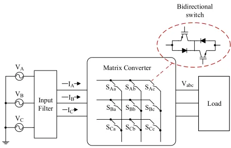
A direct matrix converter(MC) is a AC/AC converter that is capable of converting varying amplitude, fixed frequency input to varying amplitude and frequency output without employing an intermediate DC-link capacitor. Nine bidirectional voltage-blocking current-conducting switches arranged in the form of a matrix as shown in Fig. 1 constitutes a MC making it possible for bidirectional power flow. In the recent years, MCs have reached a good level of technological maturity that allows their practical and industrial implementation in a variety of applications, such as industrial drives [1-2], power supplies [3], aerospace applications [4-7]. MC is often known as an all silicon converter as there are no bulky and heavy energy storage devices [8].

The first matrix converter modulation strategy was proposed by Alesina and Venturini [9]. Even though the initial strategy proposed was capable of producing sinusoidal input and output waveforms, the maximum voltage ratio it could achieve was only 0.5. Later several other modulation techniques which produce a higher voltage transfer ratio of 0.866 such as Optimum Venturini Modulation and Space Vector Modulation (SVM) were proposed later and SVM became the most widely used modulation method for MC [10]. Since then, SVM has been applied in many applications in conjunction with feedback control strategies in order to regulate specific control variables[11].

Model Predictive Control (MPC), introduced in the late seventies [12] considers a model of the system in order to predict its future behaviour over a time horizon. A cost function represents the desired behaviour of the system. MPC is an optimization problem where a sequence of future ac-tuations is obtained by minimizing the cost function. It is also referred to as a receding horizon control, which means that at each instant the horizon is moved forward, the first

VA

VB

VC

Matrix Converter

IA

IB IC

Vabc

Load Bidirectional

switch

SAa

SBa

SCa SAb

SBb

SCb SAc

SBc

SCc Input

Filter

Fig. 1. Schematic of a direct matrix converter system

element of the sequence calculated at each step is applied at that instant and all the calculation is repeated every sample period [13]. Due to the high sampling rate used in the control of power converters, solving the optimization problem of MPC online is not practical. One approach is to use an explicit solution of MPC, solving the optimization problem offline. The resulting controller is a lookup table and can be implemented without big computational effort. Considering that power converters are systems with a finite number of states, given by the possible combinations of the state of the switching devices, the MPC optimization problem can be simplified and reduced to the prediction of the behaviour of the system for each possible state. Then, each prediction is evaluated using the cost function and the state that minimizes it, is selected. This approach has been successfully applied in recent years for the control of power converters and drives, like for current control and power control for three phase Voltage Sourse Inverters [13-14] and for current and torque control for induction motor and permanent magnet motor drives[15-17]. Even though control of currents, torque and flux are achieved, the switching frequency is variable and not fixed. MPC presents several advantages, such as fast dynamic response, easy inclusion of nonlinearities and constraints of the system, flexibility to include other system requirements in the controller, easy tuning of the control if the system model is known and the possibility of modifying and extending the methodology depending on specific applications.

introduce a modulation scheme inside the MPC algorithm [19]. However these methods involve complicated expressions for the switching time patterns and are not flexible enough to include other system requirements in the cost function. This is overcome by modulated model predictive control (M2PC) which has been proposed for a cascaded H-bridge converter [20-22], active front-end rectifier [23], two level inverter [24], three phase rectifier [25], a neutral point clamp converter [26] and indirect matrix converter [27]. Inspired from this new approach, [28] elaborates the application of M2PC for a direct matrix converter and includes experimental results to validate the simulation results discussed in [29]. This paper includes a comparison of the performance of M2PC with conventional control methods such as MPC and Proportional-Integral (PI) controller.

II. SYSTEMMODEL

In order to design the control system, an accurate model is required. The model description can be divided into matrix converter model and load model as presented in the following subsections.

A. Matrix converter model

The voltages at the output of a matrix converter and input currents are calculated from the input voltages and output currents respectively and can be derived directly from Fig. 1. The voltages and currents are represented in terms of the switching functions related to each bidirectional switch in the matrix converter as shown in equations (1) and (2).





va(t)

vb(t)

vc(t) 

= 



SAa(t) SBa(t) SCa(t)

SAb(t) SBb(t) SCb(t)

SAc(t) SBc(t) SCc(t) 

. 



vA(t)

vB(t)

vC(t) 

 (1)





iA(t)

iB(t)

iC(t) 

= 



SAa(t) SBa(t) SCa(t)

SAb(t) SBb(t) SCb(t)

SAc(t) SBc(t) SCc(t) 

 T

.





ia(t)

ib(t)

ic(t) 

 (2)

where ia(t), ib(t)and ic(t) are the output currents,

iA(t), iB(t)and iC(t)the input currents,va(t), vb(t)and vc(t)

the output voltages and vA(t), vB(t)and vC(t) the source

voltages and Sij(t)is the switching function for i= A,B and

C and j= a,b and c.

B. Load model

To determine the load current in the next sampling interval, a mathematical model of the load is required. Matrix con-verters are usually connected to an inductive load and hence this paper considers the model of a RL load to demonstrate M2PC. If M2PC needs to be implemented for MC feeding other loads such as an induction machine or a capacitive load, the load model needs to be derived appropriately. It is vital to the performance of the controller that the load model is accurate.

The continuous time model of a resistive-inductive load is given by equation (3).

Ldio(t)

dt =vo(t)−R io(t) (3) where R and L are the load resistance and inductance respectively,io(t) = [ia(t)ib(t)ic(t)]T the load currents and

vo(t) = [va(t)vb(t)vc(t)]T the matrix converter output

volt-age.

Discretising equation (3), using forward Euler approxima-tion, the discrete time model of the load can be obtained as shown in equation (4).

Io(k+ 1) = (1−

RTs

L )Io(k) + Ts

LVo(k) (4) Equation (4) is then used to predict the load currents at the future sampling instants in order to formulate the cost functions.

III. MODULATEDMODELPREDICTIVECONTROL FOR DIRECTMATRIXCONVERTER

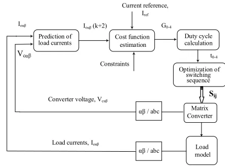
The M2PC strategy aims to combine the positive features of both SVM and MPC to obtain a model predictive control based algorithm with an intrinsic modulation scheme. A basic control block diagram of the proposed strategy for a direct matrix converter is given in Fig. 2.

Optimization of Constraints

Load

Sij Duty cycle

Matrix Prediction of

Io (k+2)

Cost function Current reference,

Iref

G0-4

/ abc Load currents, Io

Converter voltage, Vc

Vc

Io

/ abc

t0-4

load currents estimation calculation

switching sequence

Converter

model

Fig. 2. Control block diagram for M2PC strategy

A reference current is imposed upon the system and the controller is designed using the system model so that the load current tracks the reference. The measured currents are then used to predict the value of current at (k+1). The reference and predicted currents are then used to calculate the cost function which in turn is used to derive the duty cycles for the selected voltage vectors. Unlike 2-level inverters with two active and three zero vectors, matrix converter usually makes use of four active and three zero vectors to obtain sinusoidal waveforms. Active vectors are those vectors that produce a non zero voltage. Zero vectors as the name suggests does not produce any voltage.

ensured in this case as the sequence of the vectors chosen by the control will be applied within one sampling interval. The difference between a classical MPC and the M2PC is in the application time of the vectors. Unlike MPC where one vector is applied for the whole sampling interval, in the M2PC at each sampling interval; four active and three zero vectors are selected by the cost function minimization algorithm and are applied for their respective duty cycles. The active and zero vectors are then arranged in a symmetrical manner as shown in Fig. 3; to achieve minimum switching losses and reduce harmonics. The switching pattern is similar to that used in a standard SVM scheme. t01, t02 andt03 are the application times for the three zero vectors and t1, t2, t3 and t4 for the four active vectors.

Ts

V1

z3 z1 z2 z1 z3

2

t01 2

t2 2

t1 2

t3

t4 2

t02

t4 2

t3 2

t01 2

t2 2

t1 2

t03 2

t03 2

V3

V3 V4

V2 V4 V2 V1

Fig. 3. Symmetrical switching pattern for a direct matrix converter

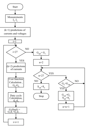
Fig. 4 shows the flowchart of M2PC algorithm incorporating delay compensation for the computation.

Fig. 4. Flowchart showing the M2PC algorithm

A. Prediction of Control Variables and Cost function calcula-tion

Similar to the MPC, the switching states are calculated based on a cost function minimization. The cost function can include different performance factors according to the control variables and to the constraints required. More than one vari-able can be controlled with the same control loop, providing

a multi-objective control approach and avoiding nested loops. In this paper, the M2PC algorithm is provisionally applied to a direct matrix converter feeding a RL load to demonstrate current control capability.

For an RL load, the prediction of load current makes use of the current measurement at the present instant or instant ’k’ and the load parameters as shown in (4). For MPC, the prediction of load current is carried out once using the optimal switching state from the previous instant. Since the M2PC incorporates a modulation scheme, more than one active vector will be applied during one sampling interval. For a direct matrix converter, out of the 27 switching states, the six rotating vectors are not considered for modulation resulting in 21 switching states to choose from. As in a standard SVM strategy [10] it is assumed that a minimum of four active vectors is required to get sinusoidal waveforms for a matrix converter. Hence the M2PC strategy will also consider four active vectors and three zero vectors to apply during one sampling interval. The predictions for four active vectors and zero vectors are done as if they were applied for the whole sampling interval. For example, for one sequence containing four active and three zero vectors, the predictions of load current are calculated as shown in equations (5) and (6). The predicted value of load current for the three zero vectors will be the same and hence it is only required to calculate once.

For active vectors :

Ioi(k+ 1) = (1−

RTs

L )I

i o(k) +

Ts

LV

i

o(k) (5)

for i=1,2,..4. For zero vectors:

Io(k+ 1) = (1−

RTs

L )Io(k) (6)

Once the currents at (k+1) instant are predicted, (k+2) predictions can be made by substitutingIo(k)withIo(k+1)in

equations (5) and (6).

Just as in MPC, the switching states are selected based on a cost function minimization. The cost function can include different performance factors according to the control variables and constraints required. More than one variable can be controlled with the same control loop, providing a multi-objective control approach and avoiding nested loops.

The cost function for load current control is essentially the error between the current demand and predicted current at (k+2) instant if the computation delay is compensated. This results in five cost functionsG0, G1, G2, G3 andG4 for each active and zero vectors. The set of quadratic cost functions can be calculated using the pre-calculated predicted currents in equation (5) as shown in (7).

Gi= (Ioref(k+ 2)−Ioi(k+ 2))2 (7)

for i=0,1,...4.

whereIoref(k+ 2)is the current demand at (k+1) instant.

algorithm is run for 18 combinations of active and zero vector sequences.

G(f inal) =G1d1+G2d2+G3d3+G4d4+G0d0 (8)

whered0, d1, d2, d3andd4 are the duty cycles for the voltage vectors.

Once the cost functions for each of the active and zero vec-tors are calculated; the predictive control will choose the best sequence of vectors which produces the lowest error. These vectors are then applied within the sampling interval with their respective duty cycles. The duty cycles are calculated based on the cost functions values of the active and zero vectors.

The multi-objective control capability of the M2PC can be achieved by simply adding the control variables to the cost function for each vector and by specifying a weighting factor for each of them. In this manner, it is possible to also consider certain constraints for the optimal operation of the system. This is demonstrated in [30] by controlling the stator currents and input reactive power of an induction motor fed by a direct matrix converter without the use of nested loops.

B. Calculation of Duty Cycles

The application times for each of the vectors are calculated from the cost functions computed for each the switching state. This method is based on the assumption that per sampling interval, the system behavior is linear in nature. From this it is possible to derive the application times for each vector as a percentage of the total sampling time. The relation between the application times of the vectors and their corresponding cost functions can be written as follows.

t=k1

G (9)

where k1 is the proportional constant and G is the cost function. Using the above equation for four active vectors and zero vector for a MC will result in a set of five equations, each dictating the application times for a particular vector in terms of the proportional constant. The condition that holds true for all the vectors applied is that the sum of the application times for all the vectors should be equal to the sampling time as shown in (10).

t1+t2+t3+t4+t0=Ts (10)

wheret1, t2, t3, t4are the times for the four active vectors and t0 is the time for three zero vectors. By substituting equation (9) in (10), the proportional constant can be obtained as shown in (11).

k1=G0G1G2G3G4Ts

A (11)

whereA= (G1G2G3G4+G0G2G3G4+G0G1G3G4+

G0G1G2G4+G0G1G2G3).

The application times for the vectors can then be derived by substituting the value of the proportional constant. The resulting set of duty cycles is shown in equation (12).

t1= (G0G2G3G4Ts)

A

t2= (G0G1G3G4Ts)

A

t3=

(G0G1G2G4Ts)

A

t4= (G0G1G2G3Ts)

A

(12)

Once the application times for active vectors are obtained, the time for zero vectors can be calculated from equation (10).

t0=Ts−(t1+t2+t3+t4) (13)

The duty cycles for each of the vector will be related to the error associated with that voltage vector. The direct relation of the duty cycles with the cost functions makes this method unique. The active and zero vectors are then applied for their respective duty cycles within one sampling interval.

The active and zero vectors are then arranged in a symmetri-cal manner as shown in Fig. 3; to achieve minimum switching losses and reduced harmonics. The switching pattern is similar to that used in a SVM scheme.t01, t02and t03 are the appli-cation times for the three zero vectors andt1, t2, t3and t4for the four active vectors in Fig. 3.

The switching frequency that can be attained using this method depends on the computational speed of the micro-processor being used. The matrix converter requires a sig-nificant computational overhead for this method since 27 switching states are available. The maximum controller update frequency obtained for M2PC within the laboratory when using a Texas Instruments C6713 DSP was 20kHz.

IV. SIMULATIONRESULTS

The M2PC is applied to a direct matrix converter feeding an RL load and simulations are done in Matlab Simulink environment to study its performance. A sampling time of

VA

VB

VC

Matrix Converter IA

IB

IC

Va

Vb

Vc

Load

abc to

Duty cycle calculation Cost function minimization Input

filter

Prediction of load currents Sij

Iref

Io(k+1) Io

Fig. 5. Control block diagram of M2PC for a matrix converter

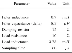
The system parameters for both the simulation and experi-mental tests are given in Table. I.

TABLE I

SYSTEMPARAMETERS

Parameter Value Unit

Filter inductance 0.7 mH

Filter capacitance (delta) 8.3 µF

Damping resistor 15 Ω

Load resistance 10 Ω

Load inductance 3.75 mH

Sampling time 80 µs

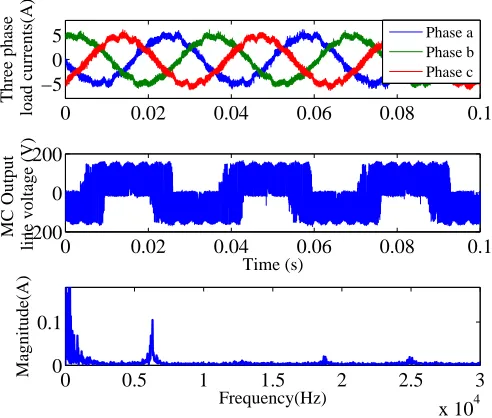
The load current of a matrix converter feeding an RL load is controlled using M2PC and the resulting waveforms are shown below. A load current reference of 5A at 30Hz is demanded from the system. Fig. 6 shows the controlled three phase load currents, MC line voltage at steady state and the Fast Fourier Transform (FFT) of the load current at steady state. It is worth noting the presence of harmonics in the range of switching frequency, 12.5kHz and its multiples. This is a result of fixed switching frequency operation. To analyse the quality of the controlled waveforms the Total Harmonic Distortion (THD) of Phase A load current is calculated and is approximately 6.3%.

0 0.02 0.04 0.06 0.08 0.1

−5 0 5

Three ph

load currents(A)

0 0.02 0.04 0.06 0.08 0.1

−200 0 200

Time (s)

MC Output

line voltage (V)

0 0.5 1 1.5 2 2.5 3

x 104

0 0.1 0.2

Frequency(Hz)

Magnitude(A)

Phase a Phase b Phase c

Fig. 6. Three phase load currents of MC controlled by M2PC

To demonstrate the fast dynamic response of M2PC, a step change from 2A to 4A and then to 2A. The resulting waveform is shown in Fig. 7 (top).

0 0.05 0.1 0.15 0.2 0.25 0.3

−5 0 5

Alpha−beta

load currents (A)

0 0.05 0.1 0.15 0.2 0.25 0.3

−5 0 5

Alpha−beta

load currents (A)

Time (s)

I

alpha Ibeta Irefalpha Irefbeta

I

alpha Ibeta Irefalpha Irefbeta

Fig. 7. Alpha-beta currents when the frequency of reference is changed

It is evident from the figure that the load current im-mediately follows the step demand in reference current and reaches steady state immediately. This indicates that M2PC can provide fast transient response which is a characteristic it inherited from MPC. In addition to the step change in current reference magnitude, a step change in the frequency of the current reference from 20Hz to 40Hz is also introduced.The resulting waveform is shown in Fig. 7 (bottom). The results indicate that M2PC is able to handle any abrupt changes in the reference signal without any overshoots or instability.

response of the M2PC controller, load current control of matrix converter is implemented using MPC and a conventional PI Controller. The system parameters for the three methods remain constant. A step demand in load current amplitude from 2A to 4A is applied to the controller and the resulting d-axis load currents with the reference signal for all the three control methods is shown in Fig. 8. To conduct a fair analysis of the transient response of the controllers considered, the PI controller is tuned to achieve very fast response to set a benchmark for the comparison.

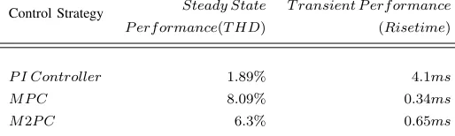
The simulation results for load current control of a direct MC with RL load are considered to compare the performance of M2PC controller with PI Controller and MPC. The THD of the currents controlled by the three methods can be considered as a measure of their steady state performance. To analyse the transient performance of the control strategies, the rise time of the controlled currents during a step change is considered. Rise time is the time taken by the control variable to reach from 10% to 90% of the steady state value. A comparison of the THDs and rise times for load current control of a MC for different controllers such as PI controller, MPC and M2PC from simulation results is tabulated in Table. II.

0.04 0.045 0.05 0.055 0.06 0.065

0 2 4 6 8

0.04 0.045 0.05 0.055 0.06 0.065

0 2 4 6 8

d−axis load current (A)

0.04 0.045 0.05 0.055 0.06 0.065

0 2 4 6 8

Time (s)

I_dref I_d

M2PC

MPC

PI Controller

Fig. 8. d-axis load current with reference during a step change in the amplitude

TABLE II

COMPARISON OFTHDS AND RISE TIMES OF LOAD CURRENTS FOR

DIFFERENT CONTROL STRATEGIES

Control Strategy Steady State T ransient P erf ormance

P erf ormance(T HD) (Risetime)

P I Controller 1.89% 4.1ms

M P C 8.09% 0.34ms

M2P C 6.3% 0.65ms

From Table. II it can be seen that PI Controller with SVM

resulted in waveforms with least harmonic distortion followed by M2PC. MPC resulted in waveforms with the worst current quality. Predictive control based algorithms such as MPC and M2PC had faster dynamic response with rise times of 0.34ms and 0.65ms respectively; compared to that of PI controller that resulted in a rise time of 4.1ms. These results prove that M2PC is capable of fast dynamic response very similar to that of MPC when compared to a traditional PI controller and deliver waveforms with enhanced current quality compared to MPC.

V. EXPERIMENTALRESULTS

To validate the simulation results discussed in the previous section, the M2PC is implemented on a matrix converter feeding an RL load in the laboratory. The parameters of the system are given in Table. I.

Fig. 9. Experimental setup

The experimental setup shown in Fig. 9 includes a matrix converter using SK60GM123 IGBT modules rated at 1200V and 60A, a current direction detection circuit for four step commutation and a clamp circuit for over voltage protection. Each IGBT module consists of two diodes and two anti-parallel IGBT connected in the common emitter configuration. There are three current sensors to measure the output currents and three voltage sensors to measure the supply voltage to the converter. The control platform includes a Texas instru-ment DSP and a FPGA card developed at Power Electronics Machines and Control (PEMC) Group, The University Of Nottingham. The M2PC algorithm is implemented on the DSP at a sampling frequency of80µs. An FPGA interface with the DSP ensures the four-step commutation of the switches. The setup is powered using Chroma Programmable AC source as indicated in Fig. 9.

10.8%. The harmonic spectrum of Phase A load current reveals harmonics in the range of switching frequency (12.5kHz) and its multiples which confirms fixed switching frequency operation. This validates the simulation results shown in Fig. 6.

0 0.02 0.04 0.06 0.08 0.1

−5 0 5

Three phase

load currents(A)

0 0.02 0.04 0.06 0.08 0.1

−200 0 200

Time (s)

MC Output

line voltage (V)

0 0.5 1 1.5 2 2.5 3

x 104

0 0.1

Frequency(Hz)

Magnitude(A)

Phase a Phase b Phase c

Fig. 10. Phase A load current, MC output line voltage and harmonic spectrum of load current at steady state

To analyse the transient behavior of the control strategy, a step demand in the amplitude and frequency of the reference current waveform is applied. A step in the amplitude of reference current waveform from 2A to 4A is applied and the frequency of the reference load current is changed from 20Hz to 40Hz and the resulting waveforms are shown in Fig. 11.

0 0.05 0.1 0.15 0.2

-5 0 5

Three phase _{load currents(A)}

Phase a Phase b Phase c

0.1 0.2 0.3 0.4 0.5

Time (s)

-5 0 5

Alpha-beta _{load currents (A)} Irefalpha Ialpha Irefbeta Ibeta

Fig. 11. Dynamic performance of M2PC during step change in the magni-tude(top) and frequency(bottom) of the reference load current

From Fig. 11, it is evident that the load currents respond to the sudden changes in amplitude and frequency instanta-neously without any delay. The results from the experimental

tests conforms to the simulation results which proves the system model and control strategy. To summarize, the load current control achieved by this method is characterized by very fast transient response as in the case of MPC and an improved steady state response due to the presence of an inbuilt modulation scheme.

VI. EFFECT OFSAMPLINGTIME ONWAVEFORMQUALITY Since the performance of MPC is largely dependant on the sampling interval, it is worth studying if this applies to the M2PC. For MPC, quality of the controlled currents are improved as the sampling interval gets smaller. To analyse the effect of sampling time on the quality of the controlled waveforms in this case the load currents, the M2PC strategy is implemented for three different sampling times such as

50µs,80µsand100µs. The quality of the controlled currents are assessed by comparing the THDs for these sampling times. Both simulation and experimental tests are conducted for three different sampling intervals or switching frequencies and the THDs of the resulting current waveforms are tabulated as shown in Table. III.

TABLE III

COMPARISON OFTHDS FORM2PCWITH DIFFERENT SAMPLING

INTERVALS

Sampling time Total Harmonic Distortion

Simulation Results Experimental Results

50µs 4.0% 7.33%

80µs 6.3% 10.8%

100µs 7.5% 12.07%

Table. III indicates that there is a considerable effect on the quality of the controlled waveforms as the sampling interval is changed. The current quality was the best when a sampling time of 50µsis considered and the worst when the sampling time is100µs. It is interesting to note that the M2PC strategy is also dependant on the sampling interval considered which is expected as it is predominantly a predictive control based method.

VII. CONCLUSION

VIII. REFERENCES

[1] Wheeler, P. W., J. C. Clare, M. Apap, D. Lampard, S. J. Pickering, K. J. Bradley, and L. Empringham. ”An integrated 30kw matrix converter based induction motor drive.” In 2005 IEEE 36th Power Electronics Specialists Conference, pp. 2390-2395. IEEE, 2005.

[2] P. W. Wheeler, J. C. Clare, D. Katsis, L. Empringham, M. Bland and T. Podlesak, ”Design and construction of a 150 KVA matrix converter induction motor drive,” Power Electronics, Machines and Drives, 2004. (PEMD 2004). Second International Conference on (Conf. Publ. No. 498), Edinburgh, UK, 2004, pp. 719-723 Vol.2. [3] P. Zanchetta, P. W. Wheeler, J. C. Clare, M. Bland, L.

Empringham and D. Katsis, ”Control Design of a Three-Phase Matrix-Converter-Based ACAC Mobile Utility Power Supply,” in IEEE Transactions on Industrial Elec-tronics, vol. 55, no. 1, pp. 209-217, Jan. 2008.

[4] L. Empringham, J. W. Kolar, J. Rodriguez, P. W. Wheeler, and J. C. Clare, ”Technological Issues and Industrial Application of Matrix Converters: A Review,” IEEE Transactions on Industrial Electronics, vol. 60, pp. 4260-4271, 2013.

[5] L. de Lillo, L. Empringham, P. Wheeler, J. Clare and K. Bradley, ”A 20 KW matrix converter drive system for an electro-mechanical aircraft (EMA) actuator,” Power Electronics and Applications, 2005 European Confer-ence on, Dresden, 2005, pp. 6 pp.-P.6.

[6] Wheeler, P. W., J. C. Clare, M. Apap, L. Empringham, L. De Lilo, K. Bradley, C. Whitley, and G. Towers. ”An electro-hydrostatic aircraft actuator using a matrix converter permanent magnet motor drive.” In Power Electronics, Machines and Drives, 2004.(PEMD). Sec-ond International Conference on (Conf. Publ. No. 498), vol. 2, pp. 464-468. IET.

[7] Lee Empringham, L. de Lillo, P. W. Wheeler and J. C. Clare, ”Matrix Converter Protection for More Electric Aircraft Applications,” IECON 2006 - 32nd Annual Conference on IEEE Industrial Electronics, Paris, 2006, pp. 2564-2568.

[8] J. Rodriguez, M. Rivera, J. W. Kolar, and P. W. Wheeler, ”A Review of Control and Modulation Methods for Matrix Converters,” IEEE Transactions on Industrial Electronic, vol. 59, pp. 58-70, 2012.

[9] A. Alesina and M. Venturini, ”Analysis and design of optimum-amplitude nine-switch direct AC-AC convert-ers,” IEEE Transactions on Power Electronics, vol. 4, pp. 101-112, 1989.

[10] D. Casadei, G. Grandi, G. Serra, and A. Tani, ”Space vector control of matrix converters with unity input power factor and sinusoidal input/output waveforms,” in Fifth European Conference on Power Electronics and Applications, 1993, pp. 170-175 vol.7.

[11] P. Wheeler, J. C. Clare, M. Apap, D. Lampard, S. Pickering, K. J. Bradley, et al., ”An Integrated 30kW Matrix Converter based Induction Motor Drive,” in IEEE 36th Power Electronics Specialists Conference, 2005. PESC ’05, pp. 2390-2395.

[12] E. F. Camacho and C. B. Alba, Model predictive control: Springer, 2013.

[13] J. Rodriguez and P. Cortes, Predictive control of power converters and electrical drives vol. 37: John Wiley and Sons, 2012.

[14] J. Rodriguez, J. Pontt, C. A. Silva, P. Correa, P. Lezana, P. Cortes, et al., ”Predictive Current Control of a Volt-age Source Inverter,” IEEE Transactions on Industrial Electronics, vol. 54, pp. 495-503, 2007.

[15] J. Rodriguez, J. Pontt, R. Vargas, P. Lezana, U. Ammann, P. Wheeler, et al., ”Predictive direct torque control of an induction motor fed by a matrix converter,” in Euro-pean Conference on Power Electronics and Applications, 2007, pp. 1-10.

[16] P. Correa, M. Pacas, and J. Rodriguez, ”Predictive Torque Control for Inverter-Fed Induction Machines,” IEEE Transactions on Industrial Electronics, vol. 54, pp. 1073-1079, 2007.

[17] T. Geyer, G. A. Beccuti, G. Papafotiou, and M. Morari, ”Model Predictive Direct Torque Control of permanent magnet synchronous motors,” in IEEE Energy Conver-sion Congress and Exposition (ECCE), 2010, pp. 199-206.

[18] H. Jiabing and Z. Q. Zhu, ”Improved Voltage-Vector Sequences on Dead-Beat Predictive Direct Power Con-trol of Reversible Three-Phase Grid-Connected Voltage-Source Converters,” IEEE Transactions on Power Elec-tronics, vol. 28, pp. 254-267, 2013.

[19] P. Antoniewicz and M. P. Kazmierkowski, ”Virtual-Flux-Based Predictive Direct Power Control of AC/DC Converters With Online Inductance Estimation,” IEEE Transactions on Industrial Electronics, , vol. 55, pp. 4381-4390, 2008.

[20] L. Tarisciotti, P. Zanchetta, A. Watson, J. Clare, and S. Bifaretti, ”Modulated Model Predictive Control for a 7-Level Cascaded H-Bridge back-to-back Converter,” IEEE Transactions on Industrial Electronics, vol. PP, pp. 1-1, 2014.

[21] L. Tarisciotti, P. Zanchetta, A. Watson, J. Clare, S. Bi-faretti and M. Rivera, ”A new predictive control method for cascaded multilevel converters with intrinsic mod-ulation scheme,” Industrial Electronics Society, IECON 2013 - 39th Annual Conference of the IEEE, Vienna, 2013, pp. 5764-5769.

[22] L. Tarisciotti, P. Zanchetta, A. Watson, P. Wheeler, J. C. Clare and S. Bifaretti, ”Multiobjective Modulated Model Predictive Control for a Multilevel Solid-State Trans-former,” in IEEE Transactions on Industry Applications, vol. 51, no. 5, pp. 4051-4060, Sept.-Oct. 2015.

[23] L. Tarisciotti, P. Zanchetta, A. Watson, J. Clare, M. Degano, and S. Bifaretti, ”Modulated model predictve control (M2PC) for a 3-phase active front-end,” in IEEE Energy Conversion Congress and Exposition (ECCE), , 2013, pp. 1062-1069.

In-ternational Conference on, pp. 2224-2229. IEEE, 2015. [25] L. Tarisciotti, P. Zanchetta, A. Watson, J. C. Clare, M. Degano and S. Bifaretti, ”Modulated Model Predictive Control for a Three-Phase Active Rectifier,” in IEEE Transactions on Industry Applications, vol. 51, no. 2, pp. 1610-1620, March-April 2015.

[26] Rivera, M., M. Perez, V. Yaramasu, B. Wu, L. Tarisciotti, P. Zanchetta, and P. Wheeler. ”Modulated model predic-tive control (M 2 PC) with fixed switching frequency for an NPC converter.” In 2015 IEEE 5th International Conference on Power Engineering, Energy and Electri-cal Drives (POWERENG), pp. 623-628. IEEE, 2015. [27] M. Rivera, C. Uribe, L. Tarisciotti, P. Wheeler and

P. Zanchetta, ”Predictive control of an indirect matrix converter operating at fixed switching frequency and unbalanced AC-supply,” 2015 IEEE International Sym-posium on Predictive Control of Electrical Drives and Power Electronics (PRECEDE), Valparaiso, 2015, pp. 38-43.

[28] M. Vijayagopal, P. Zanchetta, L. Empringham, L. De Lillo, L. Tarisciotti and P. Wheeler, ”Modulated model predictive current control for direct matrix converter with fixed switching frequency,” Power Electronics and Applications (EPE’15 ECCE-Europe), 2015 17th Euro-pean Conference on, Geneva, 2015, pp. 1-10.

[29] M. Vijayagopal, L. Empringham, L. de Lillo, L. Tarisciotti, P. Zanchetta and P. Wheeler, ”Control of a direct matrix converter induction motor drive with modulated model predictive control,” 2015 IEEE Energy Conversion Congress and Exposition (ECCE), Montreal, QC, 2015, pp. 4315-4321.