A study of solute solvent interactions in some associated liquids

A STUDY OF SOLUTE: SOLVENT INTERACTIONS IN

SOME ASSOCIATED LIQUIDS

Nicholas Martinus

A Thesis Submitted for the Degree of PhD

at the

University of St Andrews

1977

Full metadata for this item is available in

St Andrews Research Repository

at:

http://research-repository.st-andrews.ac.uk/

Please use this identifier to cite or link to this item:

http://hdl.handle.net/10023/15498

A STUDY OF SOLUTE - SOLVENT INTERACTIONS IN SOME ASSOCIATED LIQUIDS

A Thesis

presented for the degree of

DOCTOR OF PHILOSOPHY

in the Faculty of Science of the

University of St. Andrews

by

Nicholas Martinus

ProQuest Number: 10167397

All rights reserved

INFORMATION TO ALL USERS

The quality of this reproduction is dependent upon the quality of the copy submitted.

In the unlikely event that the author did not send a com plete manuscript and there are missing pages, these will be noted. Also, if material had to be removed,

a note will indicate the deletion.

uest

ProQuest 10167397

Published by ProQuest LLO (2017). Copyright of the Dissertation is held by the Author.

All rights reserved.

This work is protected against unauthorized copying under Title 17, United States C ode Microform Edition © ProQuest LLO.

ProQuest LLO.

789 East Eisenhower Parkway P.Q. Box 1346

n ii

i

im

A STUDY OF SOLUTE-SOLVENT INTERACTIONS IN SOME ASSOCIATED LIQUIDS

I

rjr-of the University rjr-of St. Andrews by Nicholas Martinus. ■ ■

'j ABSTRACT

tLi The variation of the viscosity of aqueous and non-aqueous electrolyte solutions with salt concentration has been studied fj

and the results interpreted in terms of a number of mathematical models. The effects of ion-association on the viscosity of i;

electrolyte solutions has been investigated by measuring the viscosity of aqueous solutions of some thallous salts.

The viscosities of alkali halide salts in formamide have been determined over a range of temperatures and new methods

for the division of viscosity B~ coefficients into ionic contributions have been proposed. The results of these studies have been interpreted in terms of the ion-solvent interactions.

The intermolecular interactions present in binary liquid mixtures of formamide with methanol, ethanol propan-l-ol

%

(ii)

DECLARATION

I declare that this thesis is my own composition, that the work oi which it is a record has been carried out by me, and that it has not been submitted in any previous application for a Higher Degree.

This thesis describes results of research carried out at the Department of Chemistry, United College of St. Salvator and St. Leonard, University of St. Andrews, under the

supervision of Dr. C.A. Vincent since 1st October, 1973*

(iii)

CERTIFICATE

I hereby certify that Nicholas Martinus has spent twelve terms of research work under my supervision, has fulfilled the conditions of ordinance no. (St. Andrews), and is qualified to submit the accompanying thesis in

application for the degree of Doctor of Philosophy.

CiA. Vincent

(iv)

ACKNOWLEDGEMENTS

First and foremost I would like to thank

Dr.CwA. Vincent for his continuous help and encouragement throughout the work.

My thanks go to Professor J.M. Tedder and Professor P.A.H. Wyatt for providing the research facilities and also for the award of a research grant from the Purdie fund.

I would also like to express my gratitude to Mr. C.D. Sinclair of the Department of Statistics for help with the statistical analysis in Chapter 3» and to Dr. M. Kent of the Department of Fisheries Aberdeen for help with the time domain spectroscopy work.

My thank are also due to Mr. J. Rennie and Mr. J.G. Ward for electronic and technical assistance, and to Mr. J.B. Martinus for his help with the diagrams in the

thesis.

Finally I thank my wife Liz for skilfully typing this thesis and for all the help and encouragement she has given me.

(v)

SUMMARY

The variation of the viscosity of aqueous and non-

4

been studied and the results interpreted in terms of a number of mathematical models. The effects of

ion-association on the viscosity of electrolyte - solutions has been investigated by measuring the viscosity of aqueous solutions of some thallous salts.

The viscosities of alkali halide salts in formamide have been determined over a range of temperatures and new methods for the division of viscosity B- coefficients into

ionic contributions have been proposed. The results oi these studies have been interpreted in terms of the ion-solvent interactions.

The intermolecular interactions present in binary liquid mixtures of formamide with methanol,ethanol propan-l-ol and butan-1-ol have been studied by viscosity measure­ ments over the complete concentration range. Finally the usefulness of time domain dielectric spectroscopy in

TABLE OF CONTENTS

(ii) Declaration (iii) Certificate

(iv) Acknowledgements ( v) Summary

Chapter One SOLUTION INTERACTIONS

1.1 Introduction 1

1.2 Methods of Studying Solution Interactions 3

(i) Thermodynamic Measurements 3

(ii) Spectroscopic Investigation 3

(iii)Transport Processes 6

? Two EXPERIMENTAL TECHNIQUES

2.1 Introduction 9

2.2 Poiseuille's Law 9

2.3 Theoretical Derivation of Poiseuille’s Law 10

2e^ Correction Factors 12

2.3 Viscometer Design 16

2.6 Apparatus 19

2.7 The Auto-Viscometer 20

2.8 The Programmer/Printer 21

2.9 Detectors 21

2.10 Thermostat Bath 22

2.11 Viscosity Measurements 23

2.12 Calibration of Viscometers 26

2.13 Density Measurement 31

■

--A

1

2.13

J

2*16

2.17 Propari-1-ol and Bntan-1-ol 37 1

2.18

2.19 Potassium Chloride 38 •f₁

2.20 Rubidium Iodide 38 1

2.21 Caesium Salts 38 ?

2.22 Thallous Sulphat e 38 _I

2.23

2.24 Thallous Nitrate ₃₉

_i

I

2.23 Tetrabutylammonium Iodide and Tetrapentylammonium

Iodide 39 T

Three VISCOSITY CE ELECTROLYTE SOLUTION 1

3.1 Introduction 4l

3.2 Jones -Dole Equation 42 4

3.3 The A - parameter in the Jones - Dole Equation 44 ;

3.4 The Jones - Dole B - Coefficient 46

'3.3 Extended Jones - Dole Equation 48 !

3.6 Method I 30 _■Î

3.7 Method 2 32 ■1

3.8 Method 3 33 "i

3.9 Comparison of Methods 1, 2 and 3

61

4

3.10 Incompletely Dissociated Electrolytes

62

3.11 Experimental Results 63 '

3.12 Thallous Nitrate 64

3.13 Thallous Sulphate

63

3.14 Thallous Hydroxide 66 _;;

3.13 B - Coefficients of the Ion pairs 67

i

Chapter Four VISCOSITY OF ELECTROLYTE SOLUTIONS IN FORMAMIDE

A«1 Introduction ?2

4o2 Previous Viscosity Studies of Formamide Solutions 72

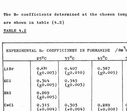
4*3 Experimental Results 73

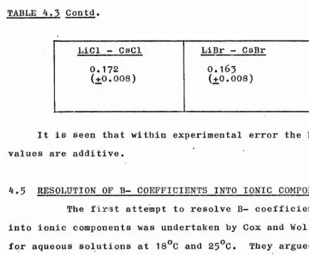
4o4 Additivity of B - ion Coefficients 78

4«3 Resolution of B •» Coefficients into Ionic

Components 79

4.6 Krumgal* z Method for Division of B Coefficients 82 4o7 B ~ Coefficients division by the correspondence

plot technique 8.5

4.8 Comparison of the Methods available for the

Division of B - coefficients 90

4*9 Ionic B - coefficients above 25^C 91

4.10 Temperature coefficient of B 97

4.11 Discussion of B- coefficients and B/ T values 97

4.12 Viscosity as a Rate Process 107

4.13 Podolsky Model ' 110

4.14 Nightingale and Benck Model 111

4.15 Feakins Model 113

4.1

6

Chapter Five SOLUTION INTERACTIONS IN ASSOCIATED

■■ LIQUIDS

5A Binary Liquid Mixtures

5.1 Introduction 122

5*2 Experimental 123 4

5.3 Results and Discussion 123

5.4 Excess Viscosity 130

5*5 Activation parameters for Viscous flow 133

5.6 Prediction of the Viscosity of Liquid Mixtures 139

5*8 Mato and Hernandez Equation

5=9 Application of Dolezalek, Tarnura«Ku rat a and Hato-Hernandez equations

5*10 Partial Mol a]. Volume

5 B Time Domain Spectroscopy

5*11 Introduction 5*12 Theory

5*15 Experimental 5*14 TDS Heasurements 5*15 Procedure

5*1

6

5*17 Conductance of the Sample 5*1

8

142

143

150

154 156

158

162 164 165 166 167

Appendix 1

Appendix 2

Appendix 3

Appendix 4

Appendix 5

Density and Viscosity of water used for viscometer

calibration

175

Thallous Nitrate, Thallous Sulphate and Thallous

Hydroxide experimental data I

76

Experimental data for electrolytes in ' \

Formamide 177

Experimental Viscosities for Binary liquid

mixtures I

83

Computer programme for Time Domain Spectroscopy

analysis and computed results for propan-1-ol 191

1.1 INTRODUCTION

The study of solution interactions has attracted attention for more than a century. Such studies fall

naturally into two categories, i.e. the investigation of electrolytic and non-electrolytic solutions.. The major drawback to the development of a completely satisfactory theory to explain solution interactions is our lack of understanding of the liquid state itself, as was pointed out as early as 1889 ^oday It is accepted that any theory of liquid solutions must be considered in relation to the structure of the solvent concerned.

Current theories of liquid structure can be divided into two main categories, lattice theories and distribution function theories. The lattice theories assume a structure similar to a certain extent to the

2 5

regular structure of a crystal e.g. Eyring , Podolsky etc. Although lattice theories are not particularly successful as predictive models on an ab initio basis they can provide good agreement with experiment when certain constants have been determined.

Distribution function theories on the other hand investigate the forces arising from interactions between moleculés and the manner in which these forces influence structure. Since liquids display only short-range order, as suggested by Samoilov , then the only quantitative way to describe liquid structure is by the construction of a radial distribution curve. This maybe achieved through X-ray and neutron diffraction studies. On the basis of these experiments, the radial distribution function of molecules is obtained from the first intensity maximum

~ 2 ”

of the radiation scattering. This function gives the probability of finding one molecule as a function of the distance from another. A knowledge of the distribution function is the minimum information required to develop

a picture of the structure of liquids. This knowledge | enables the calculation of the average distance of the

adjacent molecules and the number of nearest neighbours. However, information is required not only on the relative

positions of the molecules, but also on the forces of interaction between them. Although a general theory of intermolecular forces has not been successfully developed, various properties of these forces are known. The primary forces which keep the molecules of a liquid together are van der Waals type forces which include dispersion forces, dipole-dipole interactions, dipole-induced dipole and

hydrogen bonding. The repulsive forces between the molecules arise from the overlapping of the electron shells of the

neighbouring molecules and the mutual repulsion of the atomic nuclei. A liquid may be considered to fluctuate between a large number of equally likely structures.

Research into electrolyte solutions is currently centred on two broad areas: ion interactions and ion-solvent interactions. The study of ion-ion interactions investigates the balance of electrostatic and thermal forces and the development of models for a time-averaged distribution of ions in solution. Since the successful interionic

5

attraction theory of Debye and Hiickel a great deal of research has been concentrated in this area and refinements of their treatment of both equilibrium and transport

3

-comparison, the study oi ion-solvent interactions is

much less advanced and has not received the same attention. A large volume of work has also been carried

out on the interactions of non-electrolyte mixtures. From the initial attempt by Arrhenius ^ to predict the viscosity of binary mixtures, work has progressed to statistical

thermodynamic models and the study of thermodynamic excess functions and partial molal quantities,

1.2 METHODS OF STUDYING SOLUTION INTERACTIONS

There are perhaps three main groups of methods for studying solution interactions; thermodynamic

measurements, spectroscopic investigations and studies of transport processes.

(1) THERMODYNAMIC MEASUREMENTS

Thermodynamic properties of solutions are not only useful for estimating the feasibility of reactions in solutions, but they also offer one of the better methods of investigating the theoretical aspects of

solution structure. This is particularly true for the standard partial molal entropy, enthalpy and the partial molal volumes of the solutes, values of which are sensitive

to the arrangement of solvent molecules around a solute molecule. Enthalpies and free energies of solvation and

transfer between solvents have also been valuable in testing theoretical relationships such ,as the Born equation

The main sources of experimental data for these functions have been equilibrium studies, direct calorimetric

- 4

Solvation, two equilibria of fundamental importance are;

MX_{(a) M (soln) + X (spin)}

(

.

)

M'_{(g) + X'(g) M (solv) ^(solv) (1-2)}

These two processes are related to one another through a Born-Haber type cycle such as

“ (g) + ^(g) “ (g) X(g)

« «

•Q-f + Q

MX (S) Q soln “> M Î V + X

Q Solvation

(soln) ^(soln)

In this cycle I and A are the ionisation potential of the metal atom M and the electron affinity of the non-metal entity X respectively. is the energy or enthalpy of

the process indicated e.g.

A

(2) respectively. The thermodynamic quantities for reaction ( 1 ) are directly measurable ' and those of reaction (2)

must be calculated from

A G

solv '^°soln

A

g

A h_lattice

(1.3)

(1.4)

It is often preferable to work w i t h A c ^ a n d A H g ^ ^ y terras Since they can be divided, using certain non-thermodynamic methods, into ionic contributions, ^However A a n d

A a r e directly measurable quantities and are therefore much more accurate than the corresponding energies and

J

4

I

enthalpies of solvation. The entropies of solvation can then he calculated from

^ ^lolv

-^solv “ ~ ^

The standard entropy of solvation is given by

^ K o l v " ^ - Sg . (1-6) where is the standard partial racial entropy of the

electrolyte and is the standard molal entropy of the electrolyte in the gas phase calculated from the

Sackur-11

Tetrode equation . A good example of the use of thermo-= dynamic measurements in the study of ion-solvent interactions

1

?

is the work of" Parker et al, on the solvation of ions. In this work use was made of transference cells to determine the thermodynamics of transfer between various solvents,

(11) SPECTROSCOPIC INVESTIGATION

Spectroscopic techniques are widely used to investigate solution interactions. Much work has been

done on the selective solvation of ions by nuclear magnetic resonance spectroscopy. Infrared and Raman spectroscopy have proved invaluable in the study of hydrogen bonding and in elucidating the mechanisms of solvation. The use of dielectric .opectroscopy^ techniques is a relatively new tool in solvation studies. Time domain spectroscopy enables the permittivity and loss factor of a solvent to be determined over a range of frequency. The relaxation time of molecules can also be measured by this technique.

6

-(111)TRANSPORT PROCESSES

This covers a range of experimeatal techniques including viscosity, diffusion and electrolytic conduction studies. Information from all three sources is usefull in solution interaction studies. The measurement of the viscosity of electrolyte solutions and binary liquid mixtures was the main source of experimental results in

this project.

The theory of liquid viscosity was developed from the concepts of hydrodynamics, the study of fluids in motion. The early development of this subject took place in the eighteenth century and workers of this period were mainly concerned with so called "perfect fluids", which were characterised by the fact that they had no

tangential component of stress. Earlier, in the seventeenth I %

century Newton showed that the force F required to maintain a constant difference between two laminae with an area of contact A'was

d.v

F = TJA ---- (1.7)

d. s

where T] is called the coefficient of viscosity and is a characteristic constant for each liquid. The main development of the theory of viscous fluids was due to Navier and Stokes 1^*15 is given in standard texts

16

Classical theories of solution were built upon the analogy between the behaviour of solute particles and that of molecules of an imperfect gas. The solvent was considered to be a mere provider of the atmosphere within which the solute particles moved. Modern theories of

- 7

only the effects of tho ions on the structure of the particular solvent but also the specific ion-solvent interactions involved, A solvated ion is no longer

thought of as an ion that moves through the solution with a certain numbef of solvent molecules bound to it. A

dynamic situation is now envisaged whereby solvent molecules spend an average period of time as nearest neighbours to solute particles.

The viscosity of a liquid can be considered to be due to the interactions of the various solution species,

17

In

1929

T) /T)o =

1

+

Aci

H.

Be

(1.8)

where

7

solvent, c the concentration of solute and A and B constants characteristic of a solute in a given solvent,

Falkenhagen and Dole then showed that the Ac^ term in equation (1.8) corresponded to the ion-ion interactions

within the solution. The B factor was shown to be a measure of the ion-solvent interactions.

Thç viscosities of aqueous solutions of thallous salts and alkali halide solutions in formamide have been determined and the results considered in terms of

time-19 averaged physical models such as those of Frank and Wen and Samoilov ^ .

OQ

of components with similar molar volumes “ • Viscosity studies therefore are unlikely to yield a clear

" 9

-EXPERIMENTAL TECHNIQUES

2.1 INTRODUCTION 4

I

i

i

Of the numerous methods of measuring viscosity, I; considerations of accuracy, simplicity and susceptibility 6 to rigorous mathematical treatment have led to the

continued use and refinement of only a few.

The measurement of resistances to flow through a tube is probably still the most accurate and widely used method at the present time. Capillary viscometers

are comparatively simple and inexpensive, they require |

only a small quantity of test liquid, temperature control is easy and a full mathematical treatement is possible. In general, the liquid is made to flow through a capillary tube under a known pressure difference and the rate of flow is measured, usually by noting the time taken for a given volume of liquid to pass a graduation mark. In certain

types of instruments, the liquid is forced through the capillary at a pre-determined rate and the pressure drop produced across the capillary is measured. Capillary viscometers were used throughout this project and the

equations for laminar flow of a liquid through a cylindrical tube are derived in the subsequent sections. A full account of other methods of viscosity measurement has been given by

20 21 Dinsdale and Moore and by Swindells and coworkers *

2.2 POISEUTLLE'S LAW

Until 1842, there was little knowledge of fluid

flow through capillaries. Previous experimental investigations 09 concerning flow through tubes had been carried out by Hagen^" who used wide brass tubes in his work. . Poiseuille^*

>

10

-however, in an attempt to understand the flow of blood through the human body, undertook an exhaustive series of experiments to investigate the flow of liquid through

capillaries. He proved that the conditions of flow through

capillary tubes were much simpler than those in the wide | tubes studied previously, and showed that

Pr^

Q = K -f- (2,1)

where Q is the flux, P the applied pressure, r the radius of the capillary, 1 the length of the capillary and K a constant.

2.3 THEORETICAL DERIVATION OF POISEUILLE*S LAW

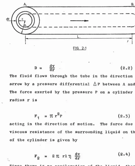
Consider a section of capillary tube of length 1, and let a liquid flow from A to B. fig (2,1)

It is assumed;

(1) that the flow is everywhere parallel to the axis (i.e. streamline);

(2) that there is no acceleration of the liquid at any point (i.e. steady flow)

(3) that there is no slip at the walls of the capillary;

(4) that the fluid is incompressible;

(5) that the fluid will flow when subjected to the smallest shearing force, the viscous

resistance being proportional to the velocity gradient.

- 11

A. B.

FIG. 2 1

D = ^ (2.2)

The fluid flows through the tube in the direction of the arrow by a pressure differential

A

F

acting in the direction of motion. The force due to the viscous resistance of the surrounding liquid on the surface of the cylinder is given by

'Ty;

'.i 't

dv (2.4)

F

2

Since there is no acceleration of the liquid, these forces must be equal and opposite, i.e.

then

Thus

dv dr V = V =

-Pr 211fl

I

-Pr^ +C

AIT]

From condition (3) ^ ' a when v 0

(2.5)

(

2

.

6

)

(2.7)

- 1 2 "

r

^ = ’»1T) (2.9)

and the velocity of the fluid is given by p » r ^

^ = 10X1 (2.10)

The velocity distribution across the capillary is there­ fore parabolic. Since v is the distance travelled in

unit time, the particles of liquid which were on the plane A at zero time will be on the surface of the parabola after unit time, in other words the volume of this paraboloid is the volume of liquid V which passes in unit time. The volume of this solid of revolution is given by

n o . Q = 2 TU

I

substituting for v _OCL

(a^ - r^) r dt (2.12) /3CL

Q =

^

o 3CL

2 2

n _ TCPaA

^ " 817) (2.13)

This formula* corresponds to the empirical Poiseuille

0"%

equation , If is the total volume of efflux in time t, the formula becomes

o _ TtPa^t

" 817] (2.14)

2.4 CORRECTION FACTORS

STREAMLINE AND TURBULENT FLOW

In the theoretical derivation of Poiseuille’s law it was assumed that the flow in the capillary was everywhere parallel to the axis. It has been found

“ 1 3 ” ■■’I

1

to be due to a change from streamline to turbulent flow. The type of flow can be characterised by a dimensionless quantity known as Reynolds Number defined by

^vd P (2.15)

" T|

where v, p and ^ are the mean velocity, the density and the viscosity of the liquid respectively, and d is the diameter of the tube. Turbulent flow normally occurs when the Reynolds number reaches-a certain value, which

experiment has shown to be about 1400 to 2000 for most capillary tubes. Flow behaviour will be the same in

different tubes with different liquids where the Reynolds Numbers are the same.

THE KINETIC ENERGY CORRECTION

Viscometers for which condition (2) page (io ) is fulfilled are characterised by very long efflux times and usually inconveniently small capillary bores. Long efflux times (in some of Poiseuille*s work one run lasted several hours) are tedious and small bores inevitably

result in difficulties due to dust particles lodging in i the capillary and altering the characteristics of the

viscometer. With most capillary viscometers, therefore, account must be taken of the work done in accelerating the liquid from rest, i.e. imparting kinetic energy. Hagenbach (i860) was the first worker to attempt to

O e nf. i

make this correction. By 1891, Hagenbach Wilberforce

27 28

Couette , and Finkener , had determined a theoretical calculation for the kinetic energy correction.

With reference to fig. (2.1) the volume of

liquid passing through the thin cylinder dr* in one second is given by:

“ lA

-I

the tube in one second. The kinetic energy of this volume of liquid is;

U = i p ( 2 T C r v dr) v^ (2.17)

or U = Tip v^r dr (2.18)

where p is the density of the liquid. From equation (2.10)

V = ^ (af - r^) (2.19)

substituting for v in (2.18), the kinetic energy given to | the liquid in time t is,

U = Ttpt (a^r - 3a^r^ + 3a^r^ - r?)dr (2.20)

Integrating between limits r = 0 to r = a gives

« = ( A t (2.21)

Now from Poiseuille’s equation (2.13) the total efflux volume in t seconds is given by

Û TCPa^* t

^ “ 8 IT) (2.22)

V

(2.23)

P 2V

41T)

TC a^t

and

( « t ] ) = ^ 3 g 1 2 ^3 (2.25)

Therefore the energy dissipated is given by equating (2.21) and (

2

25

U = ^

2

4~2

2

26

15 **

•'M

The pressure differential A P between the A and B planes fig. (2.1) is used up doing various forms of work. If P is the pressure required to overcome the forces due to the viscosity then (A P - P) is the pressure dissipated in imparting kinetic energy to the fluid. The work done in imparting kinetic energy is then (A P - P)V and as shown above

p (A P

- P)v

(A P - P) _{K a}Py2

(2.27)

(2.28)

This is a small correction which has to be deducted from the observed pressure^ difference in order to yield the pressure used in overcoming the viscosity forces.i.e. pressure used to overcome viscous iresîstance

Pv s= _{’ 4 4}

-TC a

Substitution in (2.23) gives

T)

(2.29)

4 TCa^t

81V TXPa^t

81V _

8m; t

(

2

.

30

);

(2.31)

However the actual kinetic energy correction found experimentally was

U = K..P.. 4 » (2.32)

TCPa'^t BiP V

U 81V “ 81TX t (2.33)

where m is a constant, called the Hagenbach coefficient, which depends on the viscometer characteristics. Various values of m have been deduced theoretically ranging from 0.5 (Reynolds)^^ to 1.12 (Boussinesq)^^, Experimental

16

_I

I

values of m determined, range from 0 to 1.55 with values |

around 1.12 the most prevalent. 1

COUETTE CORRECTION

In addition to the work done in overcoming the i ;i viscous resistance in the capillary itself, a small amount v? of energy is expended in overcoming the viscous forces

between the converging and diverging streamlines at the entrance and exit of the capillary respectively. The

correction for this effect takes the form of a hypothetical

increase X to the length of the capillary; equation (2,33) | then becomes

■n = ^ ( h X ) V - irfi+X )K t (2.34) The value of X cannot be deduced theoretically but must be found by experiment and is usually of the order of a few diameters.

For viscosity measurements in kinematic

instruments the pressure term P is replaced by the hydro- | static pressure head hgp to give

Ti ■

where h is the mean height of the liquid column and g is the acceleration due to gravity.

2.5 VISCOMETER DESIGN

For many of the original kinematic viscometers, which were basically glass U-tubes, difficulties arose in

I the determination of the exact mean hydrostatic pressure | head (h^gp). As flow progresses, the pressure changes ' continuously due to the drop in the height in the other "4 I :

- 17

i

1

column. The Ostwald viscometer, used for the determination of relative viscosity, simplifies matters by using a fixed volume of liquid (delivered by means of a pipette) so that the mean height of the liquid column, h^, is constant for each determination and can therefore be incorporated in a general viscometer constant.

Surface tension effects, arising from the adhesion of liquid to the walls of the bulbs immediately above the

capillary and in the exit reservoir, can also alter the | hydrostatic pressure head and give rise to uncertainties

in measurements, particularly when the surface tensions of the calibration liquid and the liquid under investigation are very different.

30 The Ubbelohde suspended level viscometer^ as used in this investigation, is considered to minimise these effects by the provision of the suspended level , at the exit of the capillary, fig. (2.2). This ’suspended level’ which is simply a bulb maintained at the same external pressure as that exerted on the liquid and of similar shape to the liquid reservoir, ensures that changes of the mean hydro­ static pressure head for the different solutions are

determined only by the density of the solution, since the pressure is maintained constant. The total volume of liquid

introduced into the viscometer does not need to be known

i

lower reservoir does not contribute to the mean hydrostatic pressure head. This is of particular advantage when .

18

19 - _I

viscometer need not be taken into account. Surface | tension effects are also minimised by use of the Ubbelohde

suspended level viscometers. At the curved surface of the bulb, at the exit of the capillary, a certain traction is developed which acts in the opposite direction

to the surface tension of the liquid in the upper bulb of the viscometer.

It is essential that the viscometer be mounted f firmly in a level position to maintain a constant hydro­

static pressure head. For a change of angle A to A + Ô A in the vertical alignment of the capillary axis, the change in the liquid head is given by

1 — cos (a — 5a ) cos A

A deviation of 0,0436 radians will therefore produce an inaccuracy of 0,1^ in the measured viscosity, Jones and

17

Dole noted that, despite their efforts to maintain a rigid reproduceable mounting for their viscometer, the efflux time changed by approximately 0,1^ over a certain period of time. The cause of this was attributed to the fact that their laboratory building was jacked up at one end to allow repairs to be carried out on the foundations i

Accurate temperature control is necessary for viscosity measurements. This is especially true for associated solvents which often have large temperature coefficients of viscosity,

2.6 APPARATUS

The viscometers used in the project were Ubbelohdé suspended level viscometers conforming to

20

-sections were approximately 80 ram long and 1,0 mm in diameter and the quantity of solution required for each

%

determination was between 10 and 15 cm • The viscometers were equipped with ground glass sockets enabling them to be stoppered firmly to the air* Size 2 viscometers were used throughout. These had efflux times of about 250s for water at

25^0

900

The efflux times were measured by means of photocell lamp assemblies coupled to a Hewlett Packard auto-viscometer 5901 B in conjunction with a Hewlett

Packard 5903 A programmer.

2.7 THE AUTO-VISCOMETER

The Hewlett Packard . auto-viscometer, model 5901 B, measured efflux times in glass capillary viscometers and

provided automatic influxing in preparation for the efflux measurement. Very accurate timing was realised, because the efflux time was measured with an electronic counter using a quartz-crystal oscillator as a time base reference. A neon display provided a digital readout that could be held for observation until released by the operator. Automatic influxing and timing eliminated errors between

operators due to differences in technique and human fatigue. The accuracy of the timer was + 0.001s. The electronic

“ 21 *’

displayed on the instrument register. The detectors also | controlled the limits of liquid transport during influx

and the release of the liquid for the efflux measurement. A constant pressure pneumatic pump provided the pressure required to force the liquid back into the upper bulb and was automatically shut off by a signal from the upper

detector when the meniscus passed on the way up. When the meniscus again passed this detector on the way down, a signal was sent to start the timer which was only stopped

when the liquid meniscus passed the lower detector. When % incorporated with the programmer printer a permanent record

of the efflux time was obtained. The auto-viscometer was equipped with four sets of detectors and could therefore accommodate four viscometers.

2 .8 THE PROGRAMMER/PRINTER

The Hewlett Packard model 5903 A programmer/

printer was an electro-mechanical apparatus which programmed the output of the 5901 B auto-viscometer and provided a

printed record of the efflux time measurements, it could program the operation of the auto-viscometer such that the measurement at any channel was repeated between 0 and 10

times with 25 second intervals between measurements. This sequence could be repeated indefinitely. The printer

recorded the efflux time for each run to 0.001 or 0,01 seconds as selected on the auto-viscometer along with a coded

identification of the programmed channel and the run number

2.9 DETECTORS

22

Hewlett Packard detection system consisted of minature tungsten lamp photocell assemblies which were contained

in water-tight blocks and firmly attached to the viscometers above and below the efflux volume reservoirs. The visco­ meters were placed in the thermostatted bath completely

immersing the detectors. With the passage of time,the detectors insulation failed causing lamp failure. This

31

system has been criticised for causing heating effects but this has not been observed here,

^ O z ?

Various workers^^* ^have used detection systems in which the light source and detector were remote from the viscometer. In the second detector system, which has s o m e similarities to that of Adolph and Siedel pairs of 1 mm glass fibre light guides (Jena Glaswerk, Schott e Gen., Mainz, No, LKF1.40) were attached to the viscometers above

and below the efflux reservoirs by nylon clamps. The light guides were led out of the thermostatted bath and into a nylon block containing pairs of infrared emitters and

detectors (Texas Instruments Ltd., TIL31 and TIL78 respectively) The auto-viscometer described previously was modified to make it compatible with this detection system. The light guide system has proved very sensitive and can be used to detect the passage of a meniscus in a capillary tube of 0,5 mm diameter.

2.10 THERMOSTAT BATH

This was a water filled bath supplied by Townson

23

-considered to be accurate to at least + 0.01 C throughout

I

;

its temperature range of lO^C to 120^C. The water in the hath was circulated over a weir and around a serpentine cooling coil which was attached to a refrigeration unit.

Coolant was pumped through the cooling coil from the ! refrigeration unit, by means of a totally immersed electric

pump controlled by a variac. Provision was also made to pass cold water, from the domestic supply, through the cooling coil for high temperature work. The cold water

flow rate was controlled by a flow meter (Rotameter 1100). I Figure (2.3) shows the flow diagram for the two cooling

systems used. Two mercury.filled glass precision thermo­ meters were used to measure the temperature. These were

total immersion thermometers supplied by Zeal Ltd. One covered the range O.O^C to 25^0 and the other from 25^C to 30°C with graduations every 0.05^C. Both these thermo­ meters were standardised at the ice point.

2.11 VISCOSITY MEASUREMENTS

For accurate measurements of viscosities in capillary viscometers there are three practical areas of importance;

(1) efflux time measurement* ; (2) temperature control;

(3) efficient cleaning of the viscometer and protection against solid particles lodging in the capillary.

The human error in the measurement of efflux

time with manually operated chronometers can now be eliminated by using electronic triggers. As early as 1933» Jones and Tally used photo-electric cells to measure efflux times

24

w Q to W

O M_>

I

§

I

§

Oœ H3 >

1-3

hi S

1-3

ffl

ffi’ CO w

s i

M

i

position of the recording apparatus^and thus changing the viscometer characteristics. An 'important advantage of the detection system used in this project was that the detectors

were firmly attached to the viscometer and were not moved s during the cleaning operation. Spurious efflux times,

caused by false triggering due to air. bubbles were in­ frequent and the efflux times did not vary by more than

0

.

02

#.

Bad triggering was usually associated with faulty mounting of the detector unit. The units were mounted

firmly by their securing screws, and in the case of the Hewlett Packard detectors, were sealed against interference from air bubbles in the water bath with a silicone sealant

(Dow Corning no. 0470-0256). A further cause of bad triggering was due to insufficient filling of the viscometers. If the

quantity of fluid was too small, air bubbles were forced into the top reservoir of the viscometer, and the timer was

activated prematurely.

In practise, the minor fluctuations in efflux time for the same solution in the same viscometer were due to variations in the bath temperature. In general viscosities were measured at only one temperature each day. The thermo­

statted bath was set to the required temperature the previous evening and given at least 8 hours to equilibrate. However

i even with these precautions, it was often found necessary to

' ■' ■ ^ ■' ■■■' ' ■■ ■ ■ ■ " XJ

- 26 - ^

f The thermometers were read with a telescope, care being

taken to ensure that the operators* eye was in line with the actual reading to avoid parallax error.

The viscometers were cleaned by flushing three times with distilled water and then three times with

analytical grade acetone and finally with a stream of dust free dry nitrogen, all of which were initially passed through a number 2 glass filter, to trap any solid particles. This procedure was followed before each viscometer was filled

with a new solution. At intervals of about three months J the viscometers were completely filled with concentrated

nitric acid and left to soak for two days. They were then washed out and filled with distilled water and soaked for about a week to ensure that no traces of acid remained,

2.12 CALIBRATION OF VISCOMETERS

Capillary viscometers may be used for absolute or relative measurements. The absolute instruments are

normally used only for the establishment of primary standards and require very accurate control of applied pressure and a precise knowledge of the capillary dimensions. Relative viscometers, as used in this project, require calibration with standard liquids.

The viscosity of freshly distilled water at 20^C has been determined by an absolute method and found to be

1,0019 X 10“ ^ 3*0 X 10~7 j The rounded off value of 1.002 X 10“ ^ J m“ ^s has been generally accepted^^ and is used as the primary calibration standard for relative viscometers.

' ,J

27

-This primary standard has been used to determine the viscosity of water at all temperatures between O^C and lOO^C and also the viscosity of aqueous sucrose solutions to be used as secondary standards^^ • The viscosity of water, between 0°C and 20^0 has been shown to follow from

the relationship

l o g T| rp ________ 1301_________________ _{998.333+8.1855 (T-20)+0.00585(T-20)^}[1-3.30233

(

2

.

36

)

and between 20°C and 100°C

1.3272 (20-T) -0.001053 (T-20)^

IT-Ï 105T --- (2.37) The Ubbelohde • suspended level viscometers used in this

work were calibrated with freshly distilled water over the temperature range 10^C -

50

temperature range, equation (2.35) can be written as

= A — B

p t ^2 (2.38)

The known viscosity and density and the measured efflux times were substituted into equation (2.38) and a plot of l/t^ against *T1 / p t was constructed, fig. (2,4) From equation (2.38) the plot should be linear, with gradient -B and intercept A, Inspection of fig, (2.4) however

indicates a slight curvature, which has also been demonstrated by McDowall , The most accurate calibration is obtained when a calibration standard of similar viscosity to the

CD

m

CM

m

CM

xr

CM

(D

CM

MT

O

th m <T>

lÔ ro

O) LO

en tr>m

29

-I higher viscosity region, 20^ and

30

efflux times for these solutions were determined and the plot of l/t^ against 1) /pt constructed, the points fell below the line indicated by the distilled water calibration fig

(2.3). The efflux times for the sucrose solutions were completely repeatable and were the same for independent freshly prepared solutions. No reason could be found for the discrepancey of the two calibration liquids. The sucrose points were eliminated from the calculation and the distilled water calibration data was extrapolated to higher viscosity regions.

As the function

_ , O (2.39)

Tfl / p t = A - B/t

was not linear, the mathematical function used to analyse the calibration data was a quadratic equation of the form

y s A+ Bx+ Cx^ (2.40)

where y =1] / p t and x = l/t^.

The coefficients for equation (2.40) were determined by regression analysis and values for these coefficients are shown in table (2.1) for two typical viscometers.

TABLÉ 2.1

VISCOMETER 1 VISCOMETER 2

A 3.59 x10~5 3,6138 X 10*5

B -8.64 xIO"^ -

1.236

10*2

0 -2.35 xIO^ -

65,00

XT

LO

ro

ro

O

04

to

to

CD

ih

ro

S

ro

ro

CD

- 31

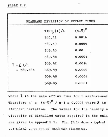
T A B L E 2.2

STANDARD DEVIATION OF EFFLUX TIMES

TIME^(t)/s (t-t)2

369.42

0.0016

369.49

0.0009

369.46

369.48 0.0004

t = Z t/n

369.42

0.0016

=s

369

46

369.49

0.0009

369

369.45

where t is the mean efflux time for n measurements. Therefore 0 = (t-t)^ / n-1 = 0.0008 where 0 is the standard deviation. The values for the density and

viscosity of distilled water required in the calibration are given in appendix 1 . Fig. (2.6) shows a typical

calibration curve for an Ubbelohde Viscometer.

2.13 DENSITY MEASUREMENT

The density of the solutions was determined using Lipkin bicapillary pycnometers . The pycnometers were constructed from 1 cm^ pipettes (Pyrex 3240/20) with graduations every 0.01 cm and had a capacity of approx. 30 cm^ fig. (2.7) • The pycnometers were calibrated with freshly distilled water at 2.5^0 intervals from 15^0 to

50^C by filling with a known weight of water and noting

32

-O

CD

CO

O

lb

CO

ID

CO mCO

•H

o

ID

O_ro

ID

O

33

'I 34 «

the limh reading at those temperatures* From the known density of water at the chosen temperatures a calibration graph of volume against total limb readings was constructed. This relationship was linear for all pycnometers used.

The data was then analysed by a least squares programme and the calibration constants for each pycnometer were computed. The left hand limb of each pycnometer was bent through an angle of approximately 140^ to allow self­

filling by syphoning. The limb readings were observed using a cathetometer. One of the calibration points near

the top of the limb was taken as the standard point and the difference between the height of the solution in the limb, and the standard point was taken as the limb reading.

% The cathetometer permitted a reading accuracy of hh 0.002 cm

%

in 30 cm of solution. Since the weighing was more accurate than this, the accuracy of the density measurements was

therefore considered to be 0.01#.

The procedure adopted for the density measurements, was to wash out the pycnometer three times with distilled water and then three times with Analar acetone. The

35

-different temperatures, in all cases, the level of the meniscus was found to be steady after five minutes

equilibration.

2.14 PREPARATION OF SOLVENT

FORMAMIDE

Formamide is a particularly difficult solvent to work with. It is thermally unstable, photosensitive and hygroscopic.

The most common method used for the purification of formamide is fractional crystallisation . Thia method however is very wasteful and inconvenient for the preparation of

large quantities.

The major impurities in commercial formamide are water and dissolved ions. A purification method

41

proposed by Notley and Spiro involving the use of ion exchange resins and molecular sieves yields formamide with the lowest recorded specific conductance (2 x 10"^S ra""^). This method of purification proved impractical for viscosity

studies since formamide prepared in this manner yielded spurious efflux times. These were considered to be due to dust particles, from the molecular sieves, lodging in

the viscometer capillaries despite filtration of the solvent. The method adopted for the purification of

“ 36

-— 2

less than 100 N m was obtained using a rotary oil pump

and a liquid nitrogen trap. The solvent formamide (re- | agent grade Hopkin and Williams) was neutralised, if

necessary, by the addition of dilute aqueous sodium

hydroxide solution to a bromothymol blue end point. The s neutral liquid was heated to 65^0 ~ 75^C under reduced

pressure, the ammonia and water pumped off, and the

formamide again neutralised. This procedure was repeated | until the liquid remained neutral when distillation began.

The solvent was then distilled repeatedly at pressures of —2

less than 100 N m . Only the middle fraction of the solvent distilling between 65^C and

70^0

42

0.025^ as determined by Karl Fischer titration, and specific conductance 2.50 x 10“^S m“ ^ .

Due to the difficulty of keeping formamide in a high state of purity, the material was used as soon as possible after purification. When formamide was not used

within seven days of preparation, it was redistilled before % use. Formamide and all formamide solutions were stored

in a cold room in the dark in ground glass stoppered flasks and sealed to the atmosphere with a paraffin film,

2.15 METHANOL

Solvent grade methanol was dried by the method of Lund and BJerrum using a Grignard type reaction^^.

20 g of magnesium turnings 0.1 g iodine and 50 cm^ methanol were allowed to react in a dry flask. When the reaction

37

distilled at atmospheric pressure, using a similar still to that described above, into a dry flask protected from atmospheric moisture. Methanol prepared in this manner was found to have a water content 6f 0.02^ as determined by Karl Fischer titration.

2.16 ETHANOL

Solvent grade ethanol was distilled with 5^ k k

benzene to remove water present • The benzene-ethanol solution formed a ternary azeotrope of benzene-ethanol-water, which distilled oyer at 64.5^0. A fractionating column similar to that used for formamide was employed to redistill the dry ethanol. The middle fraction

distilling _ at 78^0 was collected. The sample prepared thus, had a water content of 0.015^.

2,17 PR0PAN-1-0L AND BUTAN-1-0L

Reagent grade samples (Fisons Ltd.) were twice fractionally distilled through a 1 metre column packed with glass helices according to the method of Mathews and McKetta . The distillations were carried out at reduced pressure and gave final products with a boiling range of less than 0.02^C.

All the alcohols were stored in ground glass stoppered flasks sealed with a paraffin film.

2,18 PREPARATION OF SALTS LITHIUM BROMIDE

38

-1 bromide was recrystallised three times from absolute alcohol, % The white crystals were dried in a vacuum oven at 135^C

—2

and 100 N m for seven days before use,

'?

2.19 POTASSIUM CHLORIDE

Analar grade potassium chloride was used without

I

2,20 RUBIDIUM IODIDE

Reagent grade rubidium iodide was dried at 120^0 for twenty four hours and stored in vacuum over P^O^.

2.21 CAESIUM SALTS

Caesium chloride, caesium bromide and caesium

iodide were each recrystallised twice from freshly distilled water. The salts were then dried at 140°C in a nitrogen atmosphere and stored in vacuum over

P^Oy.-2.22 THALLQUS SULPHATE

Reagent grade thallous sulphate was twice re­ crystallised from boiling freshly distilled water. The needle-like white crystals were then dried in vacuum over

V 5

-2.23 THALLOUS HYDROXIDE

Solutions of thallous hydroxide were prepared by precipitation of barium sulphate from solutions of

thallous sulphate and carbonate free barium hydroxide at lOO^C, Since aqueous solutions of thallous hydroxide were

required, no attempt was made to isolate solid thallous

I

39

-■ê hydroxide or its hydrate. The concentration of the stock

solutions ( 0.3 mol dm"*^) of thallous hydroxide prepared in this manner were accurately * determined by potentiometric

titration with standard acid. More concentrated solutions { '§ of thallous hydroxide were prepared, but these tended to

produce yellow insoluble crystals of thallous hydroxide monohydrate TIOH. H^O. Other concentrations of thallous hydroxide solutions were prepared by dilution of the

stock solutions by weight.

2.24 THALLOUS NITRATE

.■s'

Thallous nitrate was prepared by precipitation frofn thallous hydroxide solution with concentrated nitric acid. The white thallous nitrate crystals were washed with small volumes of ice-cold distilled water and dried

in vacuum over PgO^.

2.25 TETRABÜTYLAMMONIUM IODIDE & ' TETRAPENTYLAMMONIUM IODIDE Both salts were used as received without furthèr purification or drying. Attempts at drying in vacuum, or over dessicants produced a brown discolouration on the

surface of the materials. The salts showed the same dis- S colouration when they were dried at 120^0 in an oven at

40

CHAPTER THREE

:tl

■ 1

-VISCOSITY OF ELECTROLYTE SOLUTIONS

3.1 INTRODUCTION

46

In 1847; Poiseuille showed that some salts increased the viscosity of water, whereas others decreased it, A r r h e n i u s m a d e some viscosity measurements on

solutions and found that the change in viscosity caused by addition of a salt was roughly proportional to the concentrations at low molarities, but increased more rapidly than the concentrations at moderate molarities. He proposed the relationship

CLl) .

where ^ the relative viscosity of the solution equal to the viscosity of the solution divided by the viscosity of the solvent, c is the concentration of the solution i

and A is a constant for any given salt and temperature, % 48

At the beginning of this century, Gruneisen measured the viscosities of electrolyte solutions down

to a very low concentration and found that, in dilute

solutions the viscosities were not linear with concentrations but showed a characteristic curvature. This curvature

was always negative i.e. the viscosity increased irrespective of whether of not at higher concentrations, the salt

increased or decreased the relative viscosities.

49