Optimization of Fairhurst Cook Model for 2 D Wing Cracks Using Ant Colony Optimization (ACO), Particle Swarm Intelligence (PSO), and Genetic Algorithm (GA)

ISSN Print: 2327-4352

DOI: 10.4236/jamp.2018.68134 Aug. 9, 2018 1581 Journal of Applied Mathematics and Physics

Optimization of Fairhurst-Cook Model for 2-D

Wing Cracks Using Ant Colony Optimization

(ACO), Particle Swarm Intelligence (PSO), and

Genetic Algorithm (GA)

Mohammad Najjarpour, Hossein Jalalifar

Department of Oil and Gas Engineering, Shahid Bahonar University of Kerman, Kerman, Iran

Abstract

The common failure mechanism for brittle rocks is known to be axial split-ting which happens parallel to the direction of maximum compression. One of the mechanisms proposed for modelling of axial splitting is the sliding crack or so called, “wing crack” model. Fairhurst-Cook model explains this specific type of failure which starts by a pre-crack and finally breaks the rock by propagating 2-D cracks under uniaxial compression. In this paper, opti-mization of this model has been considered and the process has been done by a complete sensitivity analysis on the main parameters of the model and ex-cluding the trends of their changes and also their limits and “peak points”. Later on this paper, three artificial intelligence algorithms including Particle Swarm Intelligence (PSO), Ant Colony Optimization (ACO) and genetic al-gorithm (GA) has been used and compared in order to achieve optimized sets of parameters resulting in near-maximum or near-minimum amounts of wedging forces creating a wing crack.

Keywords

Wing Crack, Fairhorst-Cook Model, Sensitivity Analysis, Optimization, Particle Swarm Intelligence (PSO), Ant Colony Optimization (ACO), Genetic Algorithm (GA)

1. Introduction

The study of rock failure under compression is a matter of importance in rock mechanics. Two main mechanisms, including axial splitting and shear failure, How to cite this paper: Najjarpour, M.

and Jalalifar, H. (2018) Optimization of Fairhurst-Cook Model for 2-D Wing Cracks Using Ant Colony Optimization (ACO), Particle Swarm Intelligence (PSO), and Genetic Algorithm (GA). Journal of Applied Mathematics and Physics, 6, 1581-1595.

https://doi.org/10.4236/jamp.2018.68134

DOI: 10.4236/jamp.2018.68134 1582 Journal of Applied Mathematics and Physics have been identified for this type of rock failure [1]. Failure by splitting mechan-ism can be related to the spalling phenomenon [2]. This phenomenon always occurs at high stress contact points, for example in a ball bearing. Spalling occurs where the maximum shear stress occurs below the rock surface.

Splitting parallel to the direction of maximum compression is a common type of macroscopic fracture of a brittle rock in the vicinity of its surface. Modelling of brittle failure is one of the greatest challenges of material failure analysis which results from the irreversible and very rapid propagation and connection of cracks, in a process called fracturing.

Materials like natural ice and rock are heterogeneous and crystalline with dif-ferent behaviors under variation of applying forces. Generally, their behavior can be categorized in two main types, including ductile behavior under high confin-ing pressures, and brittle behavior under low confinconfin-ing pressures [3]. Because most rocks are brittle at low temperature and low confining pressure, virtually most of the rocks at or near the Earth’s surface exhibits brittle failure mechan-ism. In other words, failure in these rocks occurs as deformation-induced loss of cohesion [4] [5] [6] [7].

One of the main mechanisms proposed for modelling of axial splitting is the sliding crack or “wing crack” model which was originally proposed for a 2D crack in a plate [3] [8] [9] [10]. Splitting failure begins with a primary crack (pre-crack) and then sliding mechanism creates secondary cracks or so called, wings, at the edges of those primary cracks. The macroscopic failure occur when a series of cracks extend and link together to split the material. The wedged crack can be modelled as a straight representative crack, where the wedging forces on the pre-crack area are opening the crack. This is often called the Fairhurst-Cook model [3]. The whole process of creating a 2D wing crack with Fairhurst-Cook model and an optimization process on this model is done by Dyskin et al. (1994). The basis of this optimization was the crack semi-length (l) and a critical point for this parameter found in this study which results in an un-stable mode for the crack [11]. Another Optimization on the Fairhurst-Cook model is the purpose of this paper which is the optimization of wedging force based on the crack angle to find its critical points.

2. Ultimate Rock Strength

orien-DOI: 10.4236/jamp.2018.68134 1583 Journal of Applied Mathematics and Physics tation of shear failure with confining pressure using this model are already known and presented by Nemat-Nasser and Horii (1984) [1].

As discussed before, under uniaxial compression, the tension cracks grow at a sharp angle relative to the orientation of overall failure plane with confining pressure. Variation of this “crack angle” changes the amount of wedging force with specific but different trends, resulting different amounts of opening in wing cracks and “ultimate strengths” for rocks to fail under compression. Excluding these trends is another purpose of this paper.

3. Fairhurst-Cook Model

As it can be seen in Figure 1, under uniaxial compression, crack opens in the shape of a wing with a specific crack angle (α) and also a specific crack ampli-tude (a) (This parameter is also called “half-length” or “semi-length” in other studies; but here it is called “crack amplitude” which is more proper and diffe-rentiates it from the other “semi-length” or “l”).

The amount of this wedging force (f) which creates the wing crack can be de-termined from the following equation:

f = 2.a.σ.β(α) (1) where “σ” represents the maximum principal stress, “a” represents the crack amplitude, “f” represents the wedging force and “β(α)” is a function of crack an-gle which can be determined from the following equation:

β(α) = sin2_{(α).cos(α).(1-tan(α).tan(μ)) (2)} In the above equation, “μ” represents the internal frictional angle of the rock.

4. Sensitivity Analysis

In this study, a complete sensitivity analysis performed to find the optimized amounts of parameters in Fairhurst-Cook Model. Three main parameters

DOI: 10.4236/jamp.2018.68134 1584 Journal of Applied Mathematics and Physics including crack amplitude (a), crack angle (α) and maximum principal stress (σ) and a fixed amount of 89 degrees for internal friction angle (μ) have been consi-dered in this sensitivity analysis. According to this model, these parameters have the main roles in determining the amount of wedging force which creates a two-dimensional wing crack, while the internal friction angle (μ) should be de-termined according to the rock sample which is being cracked.

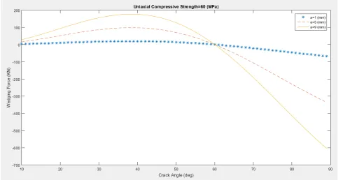
Three different stages have been considered in the sensitivity analysis process. In the first stage of this process, crack amplitude analyzed and this process re-peated for the second and third stages by analyzing crack angle (α) and maxi-mum principal stress (σ). Performing this sensitivity analysis in Matlab envi-ronment, results in Figure 2 as the output.

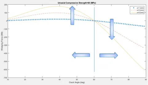
As it can be seen in Figure 2, it includes two different parts which are diffe-rentiated in a specific point. By focusing on this figure, the trend of changing the wedging force creating wing crack by variation of crack angle in different crack amplitudes can be excluded. This process is shown in Figure 3.

As it is shown in Figure 3, trends change in a certain point (α = 60.7˚). Before this point, in any crack angle, the amount of wedging force increases by increas-ing the crack amplitude, but this trend changes after this point (α = 60.7˚) and by increasing the crack amplitude, wedging force will decrease. This amount of crack angle (α = 60.7˚) virtually acts like a border line and specifies the maxi-mum amount of crack angle which causes the increase of wedging force. In other words, this specific crack angle (α = 60.7˚) has considered to be the “peak point” for crack angle in analyzing the change of wedging force by variation of crack amplitude.

DOI: 10.4236/jamp.2018.68134 1585 Journal of Applied Mathematics and Physics Another fact which can be excluded from Figure 1 is the reversion of wedging force sign from positive to negative. The reason of this conversion is thought to be the conversion of applying wedging force from tensile to compression as a result of increasing the crack angle and decreasing the angle between force di-rection and its applying area, resulting in closing of the crack lips, instead of opening. In is thought that the reason for the variation of trends is also the same, indicating that the bigger wedging force still stays bigger after peak point angle, but with a different type of force and in an apposite way, applying compression force instead of tensile and closing the crack instead of opening it. This fact highlights the importance of finding the critical angle or so called, the “peak point”.

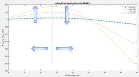
In the next stage of analyzing, the change of wedging force creating wing crack by variation of crack angle has been examined. For this purpose, one of the curves in Figure 2 has been chosen (a = 11 mm) and by focusing on it, the trend of changing the wedging force by variation of crack angle has been excluded. As it can be seen in Figure 4, this trend changes in a specific point (α = 37.7˚). Be-fore this point, by fixing the amount of crack amplitude (a) and maximum prin-cipal stress (σ), the amount of wedging force increases as the amount of crack angle increases. In other words, there is a straight proportion between these pa-rameters. After that specific point (α = 37.7˚) which is considered to be the “peak point” in variation of wedging force by changing the crack angle, that trend changes and in a reverse relation, the amount of wedging force decreases as crack angle increases. Just like the first stage, this specific amount of crack

DOI: 10.4236/jamp.2018.68134 1586 Journal of Applied Mathematics and Physics Figure 4. Different trends of changing the wedging force by variation of crack angle.

angle (α = 37.7˚) acts like a border line which limits the increase of wedging force by increasing the amount of the relevant parameter.

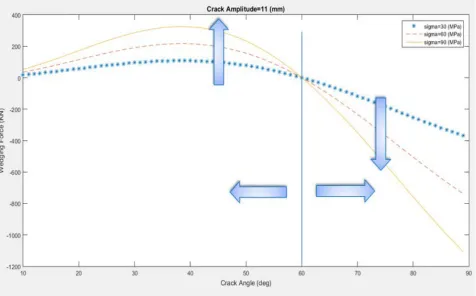
For the third stage of this sensitivity analysis which includes analyzing the wedging force variation by changing the maximum principal stress (σ), three different amounts of maximum principal stress considered in a fixed amount of crack amplitude (a). In this stage, the variation of wedging force by changing the crack angle in different amounts of maximum principal stress has been investi-gated and by its excluded trends, plotted in Figure 5 and Figure 6.

As it can been seen in Figure 6, trend of changing the wedging force by changing the crack angle in different amounts of maximum principal stress changes in a specific amount of crack angle (α = 60.7˚), like the previous stages. This point which considered to be the “peak point”, differentiates the trends and returns it from straight relation to the reverse. Just like previous stages. This peak point limits the increase of wedging force by increasing the relevant para-meter.

DOI: 10.4236/jamp.2018.68134 1587 Journal of Applied Mathematics and Physics Figure 5. Variation of the wedging force (f) by changing maximum principal stress (σ).

DOI: 10.4236/jamp.2018.68134 1588 Journal of Applied Mathematics and Physics point angle) and also to achieve the more reliable results.

5. Ant Colony Optimization (ACO)

Ant colony optimization (ACO) is a population-based metaheuristic algorithm which can be used to find approximate solutions to hard and discrete optimiza-tion problems. ACO is an algorithm for finding optimal paths that is based on foraging behavior of some ant species searching for food [15]. In this algorithm, a set of software agents called “artificial ants” search for good solutions to a giv-en optimization problem [16]. At first, the ants distribute randomly to start searching for food. When an ant finds a food source, it walks back to the colony depositing pheromone on the ground in order to mark its favorable path which should be followed by other ants. In this situation, other ants are more likely to follow that path. As more ants find a path, it gets stronger and this process re-peats so many times until there are a couple streams of ants traveling to various food sources near the colony. However, the pheromone trail starts to evaporate over time, thus its attractive strength reduces. The more time it takes for an ant to travel down the path and back again, the more time the pheromones have to evaporate [17]. Because the ants drop pheromones every time they bring food, shorter paths are more likely to be stronger, hence optimizing the “solution”. “Positive Feedback” eventually leads to all the ants following a single path. Ant colony optimization exploits a similar mechanism for solving optimization problems. To apply ACO, the optimization problem is transformed into the problem of finding the best path on a weighted graph. The artificial ants incre-mentally build solutions by moving on the graph. The solution construction process is stochastic and is biased by a pheromone model, that is, a set of para-meters associated with graph components (i.e. nodes) whose values are modified at runtime by the ants. This process is repeated many times until the stopping condition is being satisfied and a satisfactory result is achieved. The most fam-ous application of this algorithm is finding near-optimal solutions to the travel-ing salesman problem (TSP) [15] [18] [19].

6. Particle Swarm Intelligence (PSO)

op-DOI: 10.4236/jamp.2018.68134 1589 Journal of Applied Mathematics and Physics timized answer at the end of all algorithm cycles, although it is not guaranteed.

This algorithm can be summarized in four main steps, which are repeated un-til the stopping condition is satisfied:

• _{Assigning initially random positions and velocities for all of the particles in} the search-space

• _{Evaluation of the fitness of each individual particle} • _{Updating the individual and global best positions}

• _{Updating the velocity and position of each particle [22]}

In past several years, PSO Algorithm has been successfully applied in many researches and different application areas. It is demonstrated that PSO algorithm gives better results in a faster, cheaper way compared with other methods [23].

7. Genetic Algorithm (GA)

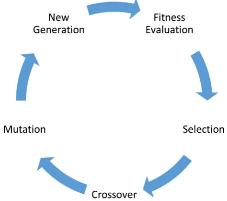
Genetic Algorithm (GA) is a heuristic optimizer algorithm based on the evolu-tionary ideas of natural selection and principles of “survival of the fittest” from “Charles Darwin”. Genetic Algorithms are commonly used to generate proper solutions to optimization problems by relying on bio-inspired operators such as “crossover” and “mutation”.

GA simulates the natural selection process among individuals (also called “phenotypes”), each of which representing a possible solution. Each possible so-lution has a set of properties and is known as a “chromosome” (also called “ge-notype”). Representing the solutions as binary strings of 0 s and 1 s are more common, but other types such as “real strings” are also applicable. The initially created individuals then lead through the process of evolution [24].

Starting with a randomly generated population of chromosomes, the evolu-tion occurs as a process of fitness based selecevolu-tion and recombinaevolu-tion to produce a better population in each iteration called a “generation” [25]. This process will be done by defining a proper “fitness function” and improving the initial popu-lation through repetitive application of the mutation, crossover and selection operators.

In each generation, the fitness of every individual in the population which is usually the value of the objective function in the problem, is being evaluated and the GA creates a new population by a new group of chromosomes with resulted fitness values. In this process, firstly, parents are selected to mate, based on their fitness, producing “offspring”, so better solutions with more fitness are given better chance to reproduce by crossover operation. The offspring inherit charac-teristics from both parents, but not equally. As parents mate and produce offspring, some new rooms must be freed for the newly generated chromosomes.

DOI: 10.4236/jamp.2018.68134 1590 Journal of Applied Mathematics and Physics generation change. Some of the individuals in the population are replaced by new ones, since the size of the population has to remain fixed and shouldn’t in-crease. The population will then consist of offspring plus a few of the older indi-viduals, which the genetic algorithm allows to survive to the next generation, because they are the best members of the population, called “elite individuals”. Following this procedure, it is hoped, but not guaranteed, that over many gener-ations, better solutions will remain while the least fit solutions die out.

Each generation will contain, on average, more good genes than the previous one. Once the population is not producing much better solutions than previous generations, the algorithm is said to have converged to a specific set of solutions for the problem. Eventually, the algorithm terminates when either it converged to a proper solution with satisfactory fitness level or a specific number of genera-tions has been produced [26] (Figure 7).

8. Optimization Process

As it has been discussed earlier, three different optimization algorithms includ-ing Ant Colony Optimization (ACO), Particle Swarm Intelligence (PSO) and Genetic Algorithm (GA) have been used in order to find the optimum or near optimum parameters influencing the wedging force which creates a wing crack. This optimization has been performed in several cases including general max-imizing and minmax-imizing of the wedging force and also separate maxmax-imizing and minimizing of this parameter, isolated in before and after the peak point angle (37.7˚).

The First algorithm was ACO and it has been performed by a colony of 46 ants trying to find the optimum amounts of crack angle (α), crack amplitude (a), maximum principal stress (σ) and frictional angle (μ) in 100 iterations. Two spe-cific upper and lower limits have been considered for each parameter in order to specify their valid range of variation. This range was from 0 to 120 degrees for

DOI: 10.4236/jamp.2018.68134 1591 Journal of Applied Mathematics and Physics crack angle, from 0 to 89.999 degrees for frictional angle, from 0.001 to 0.046 meters for crack amplitude and finally 10 to 100 mega-Pascal for maximum principal stress. The results of this optimization are illustrated in Table 1.

The second optimization algorithm was Particle Swarm Intelligence (PSO) and it has been performed in 50,000 iterations with 10,000 swarms and 4 par-ticles for each swarm, representing crack angle (α), crack amplitude (a), maxi-mum principal stress (σ) and frictional angle (μ). Just like the previous algo-rithm, two specific upper and lower limits with the same amounts have been considered for each parameter in order to specify their valid range of variation. The results of this optimization are also illustrated in Table 1.

The third and final optimization algorithm was Genetic Algorithm (GA). In this study, real genetic algorithm used and it has been performed with 200 chromosomes and 4 genes for each chromosome. These genes represented the related parameters including crack angle (α), crack amplitude (a), maximum principal stress (σ1) and frictional angle (μ) and each chromosome represented a resulting amount of wedging force (f). The optimization process repeated for 4000 iterations with the same upper and lower limits for different parameters and like the previous stages, its results is illustrated in Table 1.

These steps repeated several times, in order to achieve better results of wedg-ing force without exitwedg-ing the valid range for each parameter and as it can be seen in this table, Particle Swarm Intelligence (PSO) algorithm achieved better results with more amount of wedging force at the end. So these amounts of parameters will be more proper to use as the optimum amounts and this method is more ef-ficient in general maximizing of wedging force in wing crack model comparing to the ACO and GA algorithms. These steps have been repeated for the general minimization stage with the same ranges for the parameters. The results are shown in Table 2 which indicate that GA is the optimum method in this stage of the optimization.

Table 1. Results of the optimization algorithms in general maximization of the wedging force.

Crack Angle (α) [deg] Crack Amplitude _{(a) [m]} Maximum Principal _{Stress (σ) [Mpa]} Frictional Angle _{(μ) [deg] Force (f) [KN]} Wedging

Ant Colony Optimization (ACO) 34.658 0.045 100.000 26.000 1586.823

Particle Swarm Intelligence (PSO) 55.393 0.045 96.812 0.0886 3266.574

Genetic Algorithm (GA) 52.874 0.043 97.009 1.977 3055.086

Table 2. Results of the optimization algorithms in general minimization of the wedging force.

Crack Angle

(α) [deg] Crack Amplitude (a) [m] Maximum Principal Stress (σ) [Mpa] Frictional Angle (μ) [deg] Wedging Force (f) [MN]

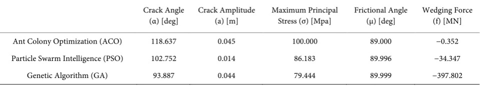
Ant Colony Optimization (ACO) 118.637 0.045 100.000 89.000 −0.352

Particle Swarm Intelligence (PSO) 102.752 0.014 86.183 89.996 −34.347

DOI: 10.4236/jamp.2018.68134 1592 Journal of Applied Mathematics and Physics As it can be understood from Table 1 and Table 2, the GA and PSO algo-rithms both had proper results with near optimum amounts of wedging forces, but ACO didn’t show any acceptable results; so this algorithm has been neg-lected in the next stages of the optimization. The results of these stages of opti-mization are shown in Table 3 and Table 4.

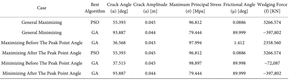
For better understanding and easier access to the best algorithms and opti-mum amounts of parameters, a summary of these methods and results are shown in Table 5. Using these optimum amounts helps to accelerate or decele-rate (in different cases of maximizing and minimizing) the opening of a wing crack by more applying wedging force in the tensile or comparison modes, avoiding the waste of time and resources.

9. Conclusions

In the first part of this study, a complete sensitivity analysis performed on the main parameters of Fairhurst-Cook Model to determine their relations and

Table 3. Results of the optimization algorithms in separate maximization of the wedging force.

State relative to the peak

point angle (37.7˚) Crack Angle (α) [deg] Crack Amplitude (a) [m] Maximum Principal Stress (σ) [Mpa] Frictional Angle (μ) [deg] Wedging Force (f) [KN]

Particle Swarm Intelligence (PSO) Before 36.684 0.046 95.710 12.878 2082.467

Genetic Algorithm (GA) Before 36.568 0.043 97.994 1.412 2358.560

Particle Swarm Intelligence (PSO) After 55.393 0.045 96.812 0.0886 3266.574

Genetic Algorithm (GA) After 52.874 0.043 97.009 1.977 3055.086

Table 4. Results of the optimization algorithms in separate minimization of the wedging force.

State relative to the peak

point angle (37.7˚) Crack Angle (α) [deg] Crack Amplitude (a) [m] Maximum Principal Stress (σ) [Mpa] Frictional Angle (μ) [deg] Wedging Force (f) [MN]

Particle Swarm Intelligence (PSO) Before 28.640 0.044 46.570 89.948 −0.490

Genetic Algorithm (GA) Before 37.515 0.045 98.897 89.998 −72.087

Particle Swarm Intelligence (PSO) After 102.752 0.014 86.183 89.996 −34.347

Genetic Algorithm (GA) After 93.887 0.044 79.444 89.999 −397.802

Table 5. Summary of best algorithms and optimum results in different cases.

Case _Algorithm Best Crack Angle _{(α) [deg]} Crack Amplitude _{(a) [m]} Maximum Principal Stress _{(σ) [Mpa]} Frictional Angle _{(μ) [deg]} Wedging Force _{(f) [KN]}

General Maximizing PSO 55.393 0.045 96.812 0.0886 3266.574

General Minimizing GA 93.887 0.044 79.444 89.999 −397,802

Maximizing Before The Peak Point Angle GA 36.568 0.043 97.994 1.412 2358.560

Maximizing After The Peak Point Angle PSO 55.393 0.045 96.812 0.0886 3266.574

Minimizing Before The Peak Point Angle GA 37.515 0.045 98.897 89.998 −72,087

DOI: 10.4236/jamp.2018.68134 1593 Journal of Applied Mathematics and Physics trends of change. Concluded results from this sensitivity analysis are summa-rized as below:

• _{The trend of changes for each of these parameters reversed in a specific}

amount of crack angle (α) as a “peak point”.

• _{This peak point is about 60.7 degrees in the analysis of crack amplitude and}

also maximum principal stress and it is about 37.7 degrees in crack angle analysis.

• _{In all of above cases, straight relations between that specific parameter and}

the amount of wedging force observed before the peak point, but it has changed to reverse relations after that point.

• _{The peak point virtually acts like a border line and limits the increase of}

wedging force by increasing the crack angle.

• _{The reason for the reversion of wedging force sign is thought to be the}

rever-sion of force from compresrever-sion to tensile with the same magnitude order; which means the biggest force still remains the biggest one, but in a reverse direction and it happens because of the changes in crack angle, making an angle of more than 90 ̊ between the direction of wedging force and its apply-ing area.

Knowing the amount of peak points can be helpful for understanding the ul-timate rock strength under uniaxial compression and also to apply optimum wedging force on a rock sample and create a wing crack. In order to achieve this optimum wedging force, a set of optimum amounts of related parameters should be used. For this purpose, three different optimizer algorithms (e.g. ACO, PSO and GA) were used and compared to identify the best algorithms and optimum results. Although it is not guaranteed that these resulted amounts of parameters are complete optimum, but they are expected to have proper applications as the local and near-global optimums with satisfactory resulting wedging force to create a wing crack.

Conflicts of Interest

The authors declare no conflicts of interest regarding the publication of this paper.

References

[1] Nemat-Nasser, S. and Horii, H. (1984) Rock failure in compression. Proceedings Ninth Workshop Geothermal Reservoir Engineering, 999-1011.

https://doi.org/10.1016/0020-7225(84)90101-0

[2] Fairhurst, C. and Cook, N.G.W. (1966) The Phenomenon of Rock Splitting Parallel to the Direction of Maximum Compression in the Neighborhood of a Surface. Pro-ceedings of the 1st International Congress of Rock Mechanics, 687-692.

[3] Kolari, K. (2017) A Complete Three-Dimensional Continuum Model of Wing-Crack Growth in Granular Brittle Solids. International Journal of Solids and Structures, Elsevier, 27-42. https://doi.org/10.1016/j.ijsolstr.2017.02.012

[4] Renshaw, C.E. and Schulson, E.M. (2001) Universal Behavior in Compressive Fail-ure of Brittle Materials. Nature, 897-900. https://doi.org/10.1038/35091045

Fail-DOI: 10.4236/jamp.2018.68134 1594 Journal of Applied Mathematics and Physics ure Mode in Ice under Low Confinement. Acta Mater, 345-355.

https://doi.org/10.1016/j.actamat.2008.09.021

[6] Horii, H. and Nemat-Nesser, S. (1985) Compression-Induced Microcrack Growth in Brittle Solids: Axial Splitting and Shear Failure. Journal of Geophysical Research, 3105-3125. https://doi.org/10.1029/JB090iB04p03105

[7] Wong, T.F. and Baud, P. (2012) The Brittle-Ductile Transition in Porous Rock: A Review. Journal of Structural Geology, 25-53.

https://doi.org/10.1016/j.jsg.2012.07.010

[8] Brace, W.F. and Bombolakis, E.G. (1963) A Note on Brittle Crack Growth in Com-pression. Journal of Geophysical Research, 3709-3713.

https://doi.org/10.1029/JZ068i012p03709

[9] Ashby, M.F. and Hallam, N.C. (1986) The Failure of Brittle Solids Containing Small Cracks under Compressive Stress States. Acta Metall, 497-510.

https://doi.org/10.1016/0001-6160(86)90086-6

[10]Horii, H. and Nemat-Nasser, S. (1986) Brittle Failure in Compression: Splitting, Faulting and Brittle-Ductile Transition. Philosophical Transactions of the Royal So-ciety A: Mathematical, Physical and Engineering Sciences, 337-374.

https://doi.org/10.1098/rsta.1986.0101

[11]Dyskin, A.V., Germanovich, L.N., Lee, K.K., Ring, L.M. and Ingrafea, A.R. (1994) Modelling Crack Propagation in Compression. Rock Mechanics, ISBN: 90 5410 380 8. [12]McClintock, F.A. and Walsh, J.B. (1963) Friction on Griffith Cracks in Rocks under

Pressure. ASME, 1015-1021.

[13]Hallbauer, D.K., Wagner, H. and Cook, G.W. (1973) Some Observations Concern-ing the Microscopic and Mechanical Behavior of Quartzite Specimens in Stiff Tri-axial Compression Tests. International Journal of Rock Mechanics and Mining Sciences & Geomechanics Abstracts, Elsevier, 713-726.

https://doi.org/10.1016/0148-9062(73)90015-6

[14]Damjanac, B. and Fairhurst, C. (2010) Evidence for a Long-Term Strength Thre-shold in Crystalline Rock. Rock Mechanics and Rock Engineering, 513-531. https://doi.org/10.1007/s00603-010-0090-9

[15]Hole, K.R., Meshram, R.A. and Deshmukh, P.P. (2015) Review: Applications of Ant Colony Optimization. International Journal of Engineering and Computer Science, 12740-12744. https://doi.org/10.5325/arthmillj.10.2.0177

[16]Dorigo, M., Maniezzo, V. and Colorni, A. (1991) Positive Feedback as a Search Strategy. Technical Report, 91-016.

[17]Dorigo, M. and Stültze, T. (2004) Ant Colony Optimization.

[18]Bonnaccorsi, A. (1992) On the Relationship between Firm Size and Export Intensity. Journal of International Business Studies, 605-635.

https://doi.org/10.1057/palgrave.jibs.8490280

[19]Deb, K., Dorigo, M., Maniezzo, V. and Colorni, A. (1996) The Ant System: Optimi-zation by a Colony of Cooperating Agents. IEEE Transactions on System, Man and Cybernetics, 29-41.

[20]Kennedy, J. and Eberhart, R.C. (2001) Swarm Intelligence (The Morgan Kaufmann Series in Evolutionary Computation).

[21]Zhang, Y. (2015) A Comprehensive Survey on Particle Swarm Optimization Algo-rithm and Its Applications. Mathematical Problems in Engineering, 1-38.

Opti-DOI: 10.4236/jamp.2018.68134 1595 Journal of Applied Mathematics and Physics mization in Text Mining. International Journal of Innovative Research and Devel-opment, 101-107.

[23]Singh, N. and Singh, A. (2012) Personal Best Position Particle Swarm Optimization. Journal of Applied Computer Science & Mathematics, 69-76.

[24]Whitley, D. (1994) A Genetic Algorithm Tutorial. Statistics and Computing, 65-85. https://doi.org/10.1007/BF00175354

[25]McCall, J. (2014) Genetic Algorithms for Modelling and Optimization. Journal of Computational and Applied Mathematics, Elsevier, 205-222.

[26]Holland, J.H. (1975) Adaptation in Natural and Artificial Systems.

Nomenclature

β(α) = model function depending on crack angle σ = maximum principal stress