Fast Computation of Pareto Set for Bicriteria Linear Programs with Application to a Diet Formulation Problem

(1)

ISSN Online: 2160-8849 ISSN Print: 2160-8830

DOI: 10.4236/ajor.2018.85019 Sep. 5, 2018 323 American Journal of Operations Research

Fast Computation of Pareto Set for Bicriteria

Linear Programs with Application to a Diet

Formulation Problem

F. Dubeau, M. E. Ntigura Habingabwa

Département de Mathématiques, Université de Sherbrooke, Sherbrooke, Canada

Abstract

In case of mathematical programming problems with conflicting criteria, the Pareto set is a useful tool for a decision maker. Based on the geometric prop-erties of the Pareto set for a bicriteria linear programming problem, we present a simple and fast method to compute this set in the criterion space using only an elementary linear program solver. We illustrate the method by solving the pig diet formulation problem which takes into account not only the cost of the diet but also nitrogen or phosphorus excretions.

Keywords

Bicriteria Linear Program, Pareto Set, Criterion Space, Weighted-Sum, Diet Formulation, Taxation System

1. Introduction

Animal diet formulation is a very important problem from an economic and environmental point of view, so it is an interesting example in operations research. Many modern animal diet formulation methods tend to take into account nitrogen and phosphorus excretions that are detrimental from an environmental point of view. Following [1], it is appropriate to apply a tax on excretions so as to change the behavior of the producers in the swine industry. These changes in behavior are studied using a formulation of the problem as a bicriteria problem and are obtained by the determination of the Pareto set of the problem. For linear models, this Pareto set is a simple polygonal line. This fact implies that changes in behavior of the producers are abrupt and correspond to particular values of the tax. In other words even in increasing the tax it can

How to cite this paper: Dubeau, F. and Habingabwa, M.E.N. (2018) Fast Computa-tion of Pareto Set for Bicriteria Linear Pro-grams with Application to a Diet Formula-tion Problem. American Journal of Opera-tions Research, 8, 323-342.

https://doi.org/10.4236/ajor.2018.85019

Received: July 26, 2018 Accepted: September 2, 2018 Published: September 5, 2018

(2)

DOI: 10.4236/ajor.2018.85019 324 American Journal of Operations Research

happen that there is no change in behavior. Behavior changes happend only at very particular values of the tax. We will see that these behaviors correspond to efficient extreme points of the Pareto set, and to every extreme point corresponds a tax interval so that any value of the tax in this interval leads to the behavior given by that extreme point.

The computation and visualization of the Pareto set, also known as the efficiency set, for bicriteria linear programming problems is a useful tool for decision makers. We could try to compute this set in the decision space [2]-[10], but due to the high dimension of this space, it can be a quite large and complicated set. Methods to obtain this set are also complicated, see for example

[11]. Fortunately, the geometric aspect of the Pareto set in the criterion (or outcome) space for bicriteria linear program is quite simple [12].

The outline of the paper is the following. The bicriteria problem is presented in Section 2. We will see in Section 3, that the Pareto set of a bicriteria linear problem is a simple polygonal line with L + 1 extreme points joined by L

adjacent segments. Then in Section 4 we presents the link between the geometric structure of the Pareto set and the weighted-sums approach. Then an elementary algorithm to determine the Pareto set in the criterion space is suggested and its complexity is analyzed. Let us point out that this method uses only elementary result from a linear program solver, that is to say the optimal solution (values of the decision variables). This fact is an interesting property of the method.

Few methods exist for computing the Pareto set in the criteria space. One such method is presented in [13]. The method requires information about the dual, assume the feasible set is compact, and determine the Pareto set with at most 2L

+ 4 calls to a linear program solver. Another simple method for bi-criteria problems is presented in [12] to obtain the Pareto set in the criterion space. The algorithm is based on information about the reduced costs of all nonbasic variables, which is equivalent to have information about the solution of the dual problem. For bi-criteria linear problems we could also use a parametric analysis to obtain the Pareto set [11] [14]. The last two methods require that the software used to solve a linear program send information about the dual, reduced cost or postoptimal analysis, which is not always possible for a simple linear program solver. Unfortunately, even if it seems that those two methods require around 2L

iterations, their complexities are nowhere analyzed. Moreover they can cycle as explained in [15] (pages 281-282), and [16] (pages 162-166).

Finally, in Section 5, we compute the Pareto sets for least cost diet formulation problems for pig, or any monogastric animal, taking into account the nitrogen and/or phosphorus excretions. Tax systems related to efficient extreme points of this problem are described.

2. Bicriteria Linear Programming Problem

Let us consider the standardform of the bicriterialinearprogrammingproblem

(3)

( )

1 1

2 2

min min suject to

0

z x c x z x c x P

Ax b x

= 

 ₌

 

 ₌



 ≥



where x is a column vector in _n_{, and the} k

c 's (k=1,2) are two row vectors

(

,1, , ,

)

k k k n

c = c _ c _in _n _{. The}_feasible _set _ _in _n _{is defined by}

{

_x n|_{Ax b}and_x 0

}

= ∈ = ≥

 , where A is a

(

m n,

)

-matrix, and b is a column vector in _m_{. Let}_C_{be the}

_{( )}

_2,_n _{-matrix given by}

1,1 1,

1

2,1 2,

2

.

n

c c

c C

c c

c

 

= =      

 

The feasible set in the criterion space _2_{is then}

{

2_| _for

}

c = z∈ z Cx= x∈ =C

  . It is well-known that  and c are

polyhedral sets in _n_and _2_{respectively. Throughout this paper we will}

suppose that the two criteria are lower bounded on  which means that for

1,2

i= _{we have}

( )

{

}

min _min _| _.

i i i

z = z x =c x x∈ > −∞

3. Structure of the Pareto Set

3.1. Efficiency Set

A feasible solution x∈ is an efficientsolution if and only if it does not exist any other feasible solution x∈ such that 1) z xi

( )

≤z xi

( )

for i=1,2, and

2) z xj

( )

<z xj

( )

for at least one j∈

{ }

1,2 . The set of all efficient solutions is

called the efficiencyset noted , also called Paretoset. The corresponding set in the criterion space is the set c=C.

3.2. Geometric Structure

Under the assumption that the two cost vectors c1 and c2 are linearly

independant, Using weighted-sums, we can replace the bicriteria linear programming problem by a single criterion linear programming problem. We consider λ∈

[ ]

0,1 _{and the weighted-sum function is}

( ) (

; 1

) ( )

1 2

( ) (

1

)

1 2 ,

z x

λ

= −

λ

z x +

λ

z x =_ −

λ

c +

λ

c x_

and we consider the single criteria problem for λ∈

[ ]

0,1

( )

(

)

subject to min

(

;

) (

1

)

1( ) 2

( ) (

1

)

1 2 .

z x z x z x c c x

P

x

λ λ λ λ λ

λ

 = − + =_ − + _

 

 _∈

 

The valuefunction ϕ λ

( )

of

(

P

( )

λ

)

is defined by

( )

min

{

z x

( )

; |x

}

.

ϕ λ

=

λ

∈

(4)

( )0,1

(

)

arg min ; .

x z x λ λ ∈ ∈ =

_

 

Hence the efficiency set  in the decision space is a connected set and is the union of faces, edges and vertices of . This set may be quite complex due to the high dimension of the decision space. On the other side c, which is the

image in _2_of __{by a linear transform, is a much simpler set.}

Since we have assumed that both criteria are lower bounded on , it follows that c is a simple compact polygonal line. Indeed in that case c is the union

of a finite number L of segments

[

Q Ql−1, l

]

[

1

]

1 ,

L

c l l

l

Q Q− =

=

_



where

[

]

{

2

(

)

[ ]

}

1, | 1 1 for 0,1 ,

l l l l

Q Q− = Q∈ Q= −

σ

Q− +

σ

Q

σ

∈

and such that

(

Q Ql−1, l

)



(

Q Ql−1, l

)

= ∅ if l l≠,

with

(

)

{

2

(

)

( )

}

1, | 1 1 for 0,1 .

l l l l

Q Q− = Q∈ Q= −

σ

Q− +

σ

Q

σ

∈

To each segment is associated a weight λl l−1, such that the vector

(

1 1,, 1,

)

t l l l l

λ₋ λ₋

− _{is orthogonal to the segment}

[

Q Ql−₁, l

]

in 2. To each point

Q of c is associated an interval Λ

( )

Q defined by

( )

(

)

(

) (

)

1, 1, 1

, if 0, , ,

, if , 1, , ,

l l

l

l l l l l l

Q Q l L

Q

Q Q Q l L

λ λ

λ− λ− −

  = =  

Λ = 

  ∈ =      where 0 1 1, 0,

for 1, , ,

1,

l l l l

L

l L

λ

λ λ λ λ − − =   ₌ ₌ ₌   ₌  

with λ λl− l>0 for l=0, , L.

3.3. Weak Efficiency Set

We will call weakefficiencyset, or weakParetoset, the set defined by

[ ]0,1arg min

( )

; .

f

x z x

λ λ ∈ ∈ =

_

 

Obviously _{ }_⊆ f _{. In the criteria space we will have} f f c =C   . Geometrically in the criterion space _2_{, this means we add to}

c

 possibly a vertical segment or a ray from Q0 in the positive direction of z2, D0=

( )

0,1 ,

(

0; 0

)

{

0 0|

(

0, 0

]

}

c,

R Q D = Q +

η

D

η

∈

η

⊂

and/or a horizontal segment or a ray from QL in the positive direction of z1,

( )

1,0

L

(5)

(

L; L

)

{

L L|

(

0, L

]

}

c,

R Q D = Q +

η

D

η

∈

η

⊂

where η0 and ηL are nonnegative finite or infinite values. They are the

maximal values of η such that R Q D

(

0; 0

)

and R Q D

(

L; L

)

are both subsets

of c. To these points on c we set

( )

[ ]

(

)

[ ]

(

0 0

)

0,0 if ; ,

1,1 if L; L .

Q R Q D Q

Q R Q D

 ∈

 Λ = 

∈ 

3.4. Link to Parametric Analysis

The parametric analysis is based on the weighted-sum given by

(

;

)

1

( )

2

( )

z x µ =z x +µz x

for µ∈

[

0,+∞

)

, and the value function in this case is defined by

( )

min

{

z x

(

; |

)

x

}

.

ϕ µ

 = 

µ

∈

Instead of

(

P

( )

λ

)

, we could consider the single criteria problem for

µ

≥0

( )

(

)

subject to min

(

;

)

1

( )

2

( ) (

1 2

)

.

z x z x z x c c x

P

x

µ µ µ

µ = + = +     _∈   

Since λ_and µ_{are related by the formulae}

and , 1 1 µ λ λ µ µ λ = = + −

to the efficient extreme points

{ }

Q_{l l}L₌₀ on the efficiency set c correspond also

the following intervals for the parameter µ

( )

(

)

(

) (

)

1, 1, 1

, if 0, , ,

, if , 1, , ,

l l l

l l l l l l

Q Q l L

Q

Q Q Q l L

µ µ

µ− µ− −

  = =  

Λ _{= }

  ∈ =       where 0 1 1, 0,

for 1, , ,

.

l l l l

L

l L

µ

µ µ µ µ − − =   = = =   _{= +∞}  

In many applications, the parameter µ is in fact a tax over the the second criteria (for a minimization problem). Interesting enough is to observe that the behavior change (extreme point) only for the critical values µl l−1, of the

parameter µ_{. Indeed when}µ_{increases and its value passes through}µ_{l l}₋_1,_,

the optimal point, extreme point, move from Ql−1 to Ql. Thus, any level of

taxes µ_{strictly between the values} µ_{l l}−_1, =µ_l and µl l, 1+ =µl causes the same

behavior described by Ql.

4. Computation of the Pareto Set

4.1. Preliminaries

(6)

( ) (

1

)

₁ ₂.

Q z z

ϕ λ = −λ +λ

Then the value function ϕ λ

( )

associated to

(

P

( )

λ

)

_{is such that}

( )

{

( )

}

( )

{

}

( )

{

}

min |

min _l | 0, , .

Q c

Q Q Q

l L

ϕ λ ϕ λ ϕ λ ϕ λ

= ∈

= = 

 

Hence we have the following results.

Theorem 4.1. [12] Let Q∈c, we have ϕ λ

( )

=ϕ λQ

( )

if and only if

( )

Q

λ∈ Λ .

Theorem 4.2. [12] Let Q∈c and 0≤λ λ1< 2≤1 . Then λ1 and

( )

2 Q

λ ∈ Λ if and only if

[

λ λ1, 2

]

⊆ Λ

( )

Q . It follows that Q is oneof the Ql

(l∈0, ,_ L_).

Theorem 4.3. [17] Thefunction ϕ λ

( )

iscontinuous, piecewise linear and

concave. The abscissae of slope changes are the increasing values λl l−1, for

1, ,

l= _ L_.

Let us observe that the slope associated to ϕ λQ

( )

strictly decreases for Q

going from Q0 to QL on c, since z1 increases and z2 decreases steadily.

We deduce the next results.

Theorem 4.4. [12] Let Qi′ and Q′j be two distinct points on c. For

[ ]

0,1

λ∈ _,

(

1−

λ λ

,

)

t _is _orthogonal _to _the _segment Q Qi′ ′, j if and only if

( )

i j

Q Q

ϕ λ

′ =

ϕ

′

λ

.

Theorem 4.5. Let Qi′ and Q′j betwodistinctpointson c and λ∈

[ ]

0,1 ,

suchthat

(

1−

λ λ

,

)

t isorthogonaltothesegment Q Qi′ ′, j. Forafixed λ, the

function ϕ λQ

( )

isconstantasafunctionofQonthesegment Q Qi′ ′, j. Letus

notethisconstantvalueby

ϕ

Q Qi j′ ′. Moreover

1) if

ϕ λ

( )

=

ϕ

Q Q_{i j}′ ′ then Q Qi′ ′, j ⊂ c, λ∈ Λ

( )

Qi′ and

λ

∈ Λ

( )

Q′j ;

2) if

ϕ λ

( )

>

ϕ

Q Q_{i j}′ ′ then

(

Q Qi′ ′, j

)

c= ∅.

Theorem 4.6. Let Qi′ and Q′j betwodistinctpointson c. If λ∈ Λ

( )

Qi′

is such that

ϕ λ

( )

=

ϕ

Q′j

( )

λ

then

λ

∈ Λ

( )

Q′j . Moreover there exists

{

0, ,

}

l∈  L suchthat λ λ= l l−1, and Q Qi′ ′, j ⊆

[

Q Ql−1, l

]

⊆c.

Theorem 4.7. Let Qi′ and Q′j be two distinct points on cf . Let

( )

i Qi

λ′∈ Λ ′ and

λ

′j∈ Λ

( )

Q′j , andconsiderthefollowingtwolines

( )

{

2_|

( )

}

i

λ

i′ = Q∈

ϕ λ

Q i′ =

ϕ λ

i′



and

( )

{

2_|

( ) ( )

}

_. j λj′ = Q∈ ϕ λQ ′j =ϕ λ′j



(A) If λ λi′≠ j′ , the point of intersection of i

( )

λi′ and j

( )

λ

′j is

(

i, j

)

(

0; ,i j

) (

, 1; ,i j

)

Q λ λ′ ′ = ψ λ λ ψ′ ′ λ λ′ ′ _where

(

; ,

)

j

( )

i

( )

,

i j i j

j i j i

λ λ λ λ ψ λ λ λ ϕ λ ϕ λ

λ λ λ λ

′ − − ′

′ ′ = ′ + ′

′− ′ ′− ′

(7)

(

0; ,

)

j

( )

i i

( )

j

i j

j i j i

λϕ λ λ ϕ λ

ψ λ λ

λ λ λ λ ′ ′ ′ ′

′ ′ = − ′− ′ ′− ′

and

(

1; ,

)

j 1

( )

1 i

( )

.

i j i j

j i j i

λ λ

ψ λ λ ϕ λ ϕ λ λ λ λ λ

′ − − ′

′ ′ = ′ + ′

′ ′ ′

− −

(B) If λ λi′= ′j, then i

( )

λ

i′ =j

( )

λ

j′ which contains the segment Q Qi′ ′, j .

4.2. Algorithm

In this section we consider both criteria upper bounded on  . In the forthcoming algorithm we initialize the process with the two points Q0 and

L

Q on c. Then we gradually obtain a sequence of points

{ }

0

I i i

Q′ ₌ _on _c, and a sequence of intervals associated to these points

{

( )

}

0

, I

i i i

i

Q

λ λ

=

 ′  ′ ′ ′

Λ =_ _ _such

that Λ′ ′

( )

Qi ⊆ Λ

( )

Qi′ and

( )

Q_i

( )

for all

( )

Qi .

ϕ λ

=

ϕ λ

′

λ

∈ Λ′ ′

At the end of the process I L= and we have Q Ql′ = l with

( )

, ,

l l Ql Ql l l

λ λ λ λ

 _{′ ′}_{= Λ}_{′ ′} _{= Λ} _{= }_ __  

for l=0, , L I= .

Algorithm (Pareto bicriteria) STEP 0. Initialization.

(A) Enter the data of the problem. (B) Determine * _{arg min}

( )

i x i

x = ∈z x for i=1,2 and set zimin =z xi

( )

* . For

, 1,2

i j= _and j i≠ _set

( )

* |

j i j i

z =z x _{. We get the initial point}

(

min

)

0 1 , 2|1

Q = z z

which as the same first coordinate as Q0, and QL=

(

z z1|2, 2min

)

which as the

same second coordinate as QL. Those two points might not be on c, but are

on f c  .

(C) Set Q0′ =: Q0 and Λ′ ′

( )

Q0 =_λ λ0′, 0′_: 0,0=

[ ]

;

(D) Set Q1′ =: QL and Λ′ ′

( )

Q1 =_λ λ1′, 1′_: 1,1=

[ ]

;

(E) Set I: 1= _.

STEP 1. As long that there exists an index i such that

λ λ

i′− i′−1>0, select one

such index i and do: (A) Find *

1,

i i

λ ∈_λ λ′− ′_ such that 1 1

( )

* _: * *

i i i i

Q Q Q Q

ϕ

′₋ ′ =

ϕ

′₋

λ

=

ϕ λ

′ , hence

[ ]

* _0,1

λ

∈ such that

(

₁₋_{λ λ}*_, *

)

t_{is orthogonal to the segment}

[

]

1, i i Q Q′− ′ (see

Theorem 4.4);

(B) Solve

(

_P

( )

_λ*

)

_{, compute}

(

* *

)

*: 1 , 2 c

Q z zλ λ

λ = ∈ with

( )

*

( )

* *

Q_λ

ϕ λ =ϕ λ _;

(C) Update the list of points

{ }

Q_{i i}′ I₌₀_{and their intervals}

( )

{

i i, i

}

I₀

i

Q

λ λ

=

 ′  ′ ′ ′ Λ =_ _ _:

I) Modification of the intervals. If

( )

* * ₁

i i

Q Q

ϕ λ

=

ϕ

′₋ ′ then all the segment

(8)

(see Theorems 4.1 and 4.5)

( )

1

* 1 *

for ,

for , .

i

Q i

ϕ λ λ λ λ ϕ λ

ϕ λ λ λ λ

−

′ −

′

 _∈ ′ 

 _ _

= 

 _{∈ } ′_ 

We modify as follow:

a) for Qi′−1: Λ′ ′

( )

Qi−1 =_λ λ′i−1, i′−1 _{ }:= λ λi′−1, *_;

b) for Qi′: Λ′ ′

( )

Qi =_λ λ′i, i′_:= λ λ*, i′;

In the sequel no more point will be generated on

[

Q Qi′−1, i′ ⊆

]

c.

II) Point insertion and interval modification. If

( )

1

* *

i i

Q Q

ϕ λ

<

ϕ

′₋ ′ then

[

]

* i1, i

Q_λ ∉ Q Q′− ′ , insert the point and modify intervals as follows (see Theorem

4.6):

a) Insert Q_λ* between Qi′−1 and Qi′ in the list with

( )

Q_λ* λ λ*, * : λ λ*, *

′

Λ =_ _ _{= } __;

b) Set I I:= +1_;

c) If ϕQ_λ*

( )

λi′−1 =ϕQi′−1

( ) ( )

λi′−1 =ϕ λi′−1 , then Q Qi′−1, λ*⊆c and any

* 1,

i

λ

∈ 

λ λ

′−  is in Λ′

( )

Q_λ* , hence we modify Λ′

( )

Q_λ* by setting λ*:=λi′−1;

d) If

ϕ

Q_λ*

( ) ( ) ( )

λ

′i =

ϕ λ

Qi′ i′ =

ϕ λ

′i , then Q Qλ*, i′ ⊆ c and any

*_,

i

λ_∈λ λ′  

is in Λ′

( )

Q_λ* , hence we modify Λ′

( )

Q_λ* by setting

λ

*:=

λ

′i.

STEP 2. For any i such that

λ λ

i′ − =i′ 0, remove Qi′ from the list and set

: 1

I I= − _.

STEP 3. End of the process (and I L= ). The output is the list

{

Ql;λ λl, l

}

_lL₌₀.

Let us observe that this process use only optimal solutions of

(

P

( )

λ

)

_,

optimal values of the decision variables, which is easily obtained from any elementary linear program solver.

Remark 4.8. Thisalgorithmproducesateachiterationaninnerandanouter

approximation. Theinner approximationis the polygonalline joiningthe Qi′

for i=0, ,_ I_._The_outer_{approximation}_is_the_polygonal_line_joining_the_points

0

Q′_, Q

( )

λ λ′₀′, ₁ _, _Q₁′_, Q

( )

λ λ′₁′, ₂ _, _Q₂′_,__, _Q_I′₋₂_, Q

(

λ

I′−₂,

λ

′I−₁

)

, QI′−1,

(

I 1, I

)

Q λ λ′− ′ , QI′, aslongasthe Q

(

λ λi′−1, ′i

)

’sarewelldetermined (seeTheorem

4.7). Attheendofthealgorithmthetwoapproximationsagree.

4.3. Complexity

In this section we are going to determine the maximum number of calls to a linear program solver to completely determine the Pareto set, or equivalently its

1

L+ efficient extreme points

{ }

Q_{l l}L₌₀. The result is given in the last theorem of this section and says that it takes at most 2L+3_{calls to a linear program}

solver to generates the L+1 extreme points

{ }

Q_{l l}L₌₀. We will use the following ordering on f

c

 . For any two distinct points Qi′

and Q′j on cf, we will say that Qi′ precedes Q′j on cf, or equivalently

(9)

DOI: 10.4236/ajor.2018.85019 331 American Journal of Operations Research 0

Q to QL we move from Qi′ to Q′j. We will note Qi′< Q′j or equivalently j i

Q′>_Q′_.

Theorem 4.9. Thealgorithmgeneratesatmost 3 pointson

[

Q Ql−1, l

]

on c

andtwoofthesepointsare Ql−1 and Ql.

Proof. Let us remark that the algorithm will eventually find a point in

[

Q Ql−1, l

]

for any l=1, , L. Let Q1 be the first point generated by the

algorithm in

[

Q Ql−1, l

]

. This first point can be generated at STEP 0, an initial

point, if Q Q0= 0∈

[

Q Q0, 1

]

for l=1 or QL =QL∈

[

Q QL−1, L

]

for l L= .

Otherwise, it is generated through STEP 1-C-II, with Qi′ <−1 Ql−1 and Ql <Qi′.

Then this point is included in the list, and there are three cases to study:

1) Q Q1= l−1=Q_λ* for a

λ

*∈ Λ

( )

Ql−1 =

λ

l−1=

λ

l− −2, 1l ,

λ

l−1=

λ

l l−1,  and we

have _Λ_′

( )

_Q1 _

_{λ λ}

**_, *_

=   with λ**≤λ*. We will have λ**=λ*, or

λ

**=

λ

l− −2, 1l

if the lower bound is modified through STEP 1-C-II-c (if Qi′ ∈−1

[

Q Ql−2, l−1

)

and

(

)

2, 1 1

l l Qi

λ_{− −} ∈ Λ′ ′₋ ).

2) Q Q Q1= l= _λ* for a

λ

*∈ Λ

( )

Ql =

λ

l=

λ

l l−1,,

λ λ

l = l l, 1+ and we have

( )

_Q1 _

_{λ λ}

*_, **_

′

Λ _{= } __with _λ*_≤_λ**_{. We will have}_λ**₌_λ*_{, or} ** , 1

l l

λ

=

λ

+ if the

upper bound is modified through STEP 1-C-II-d (if Qi′∈

(

Q Ql, l+1

]

and

( )

, 1 l l Qi

λ ₊ ∈ Λ′ ′ _).

3) 1

(

)

1,

l l

Q ∈ Q Q− for

λ

*=

λ

l l−1, and we have Λ′

( )

Q1 = 

λ λ

*, *.

Let _Q2_{be the second point generated by the algorithm in}

[

]

1, l l Q Q− . Q1

must be one of the two points used to generate _Q2_{, and hence} * 1,

l l

λ

≠

λ

− . This

point _Q2_{is generated through STEP 1-C-II, and it is included in the list. There}

are two cases to study:

1) Qi′ <−1 Ql−1 and Q Qi′ = 1∈

(

Q Ql−1, l

]

, we will have

λ

*<

λ

l l−1, and

)

( )

*

1 1, 1

1, l l l l

l Q

λ

∈

λ λ

− − =

λ

− ⊂ Λ − . Consequently Q2=Qλ*=Ql−1 and

( )

_Q2 _

_{λ λ}

**_, *_

′

Λ _{= } __with _λ**_{modified as in the preceding case. Moreover if}

( )

1 1,

l l Q

λ

− ∈ Λ′ we will modify the upper bound to get Λ′

( )

Q2 = 

λ λ

**, l l−1,.

2) 1

[

)

1 1,

i l l

Q′ =− Q ∈ Q Q− and Qi′ >Ql, we will have

* 1,

l l

λ

>

λ

₋ _and

(

( )

*

1,,

l l l l

l Q

λ

∈

λ

=

λ

−

λ

⊂ Λ . Consequently Q2=Qλ*=Ql and

( )

_Q2 _

_{λ λ}

*_, **_

′

Λ _{= } __with _λ**_{modified as in the preceding case. Moreover if}

( )

1 1,

l l Q

λ

− ∈ Λ′ we will modify the lower bound to get Λ′

( )

Q2 = 

λ

l l−1,,

λ

**.

Two points of

[

Q Ql−1, l

]

are now in the list. We can have a point

(

l 1, l

)

Q′∈ Q Q− with Λ′ ′

( )

Q = 

λ

l l−1,,

λ

l l−1, or an extreme point Ql−1, with

(

Ql−1

)

λ λ′l−1, l l−1, 

′

Λ =_ _, or Ql, with Λ′

( )

Ql = 

λ

l l−1,,

λ

l′. Otherwise the two

points are the extreme points Ql−1 and Ql. In that case, if Qi′ =−1 Ql−1 and

i l

Q Q′ = _{, it can happen that}λ λi′− i′−₁=λl l−_1, −λl l−_1, =0 and we will have

terminated with the interval

[

Q Ql−1, l

]

. Otherwise let us note Q3 the third

point generated in

[

Q Ql−1, l

]

. There are two cases to study:

1) We have only one extreme point Ql−1, or Ql, of the segment in the list

and Q′∈

(

Q Ql−1, l

)

. As in the preceding paragraph, we will introduce it in the list,

and depending of the case, by passing through STEP 1-C-II, 3 1 l Q =Q− if

1 1

i l

(10)

we will have respectively Λ′

(

Ql−1

)

=_

λ λ

′l−1, l l−1,_⊆ Λ

(

Ql−1

)

or

( )

Ql

λ

l l−1,,

λ

l

( )

Ql

′  ′

Λ =_ _⊆ Λ _.

2) We already have two extreme points Ql−1 and Ql in the list. In that case

1 1

i l

Q′ =− Q− and Q Qi′ = l and we will have

λ

*=

λ

l l−1, and Q_λ*∈

[

Q Ql−1, l

]

. We

pass through STEP 1-C-I and we modify the intervals to get

(

Ql−1

)



λ λ

′l−1, l l−1,

(

Ql−1

)

′

Λ =_ _⊆ Λ et Λ′

( )

Ql =

λ

l l−1,,

λ

l′⊆ Λ

( )

Ql . Since

1 1,

l l l l

λ

′ =−

λ

− =

λ

′, Q3=Q_λ* is not added to the list.

In the sequel, the algorithm generate no more point on

[

Q Ql−1, l

]

because if

we have two points Qi′ =−1 Ql−1 and Q Qi′ = l we have λ λi′− i′−1=λl l−1, −λl l−1, =0,

or else, if we have three points, Qi′ =−1 Ql−1 and Qi′∈

(

Q Ql−1, l

)

and Qi′ =+1 Ql

we have

λ λ

i′− i′−1=

λ

l l−1, −

λ

l l−1, =0 and

λ

′i+1− =

λ λ

i′ l l−1, −

λ

l l−1, =0.

Theorem 4.10. If Q0 <Q0, respectively QL>QL, then Q0, respectively L

Q , is eventually removed of the list without any supplementary call to the

linearprogramsolver.

Proof. When Q0 is introduced in the list, there is no supplementary call for 0, 0

Q Q

 

 . Similarly for the interval Q QL,L when QL is introduced in the

list. The points Q0 and QL are removed from the list at STEP 2 since

( )

Q0

[ ]

0,0

′

Λ  = and Λ′

( )

QL =

[ ]

1,1 .

Theorem 4.11. The algorithm generates the extreme points

{ }

L₀ l l

Q ₌ of the

Paretosetinatmost 2L+3 _calls_to_a_linear_program_solver_.

Proof. The initialization STEP 0 requires 2 calls. For STEP 1, as we generate the Ql for l=0, , L and possibly one supplementary call for each segment

[

Q Ql−1, l

]

for l=1, , L, there is at most 2L+1 calls. Hence the algorithm

requires at most 2L+3_calls.

5. A Real World Application: Pig Diet Formulation

To illustrate our method of computation of the Pareto set we consider the pig diet formulation problem taking into account not only the cost of the diet but also environmental considerations, such as the reduction of nitrogen or phosphorus excretions. One way to analyze this problem is to rewrite the problem as bicriteria problem. Hence the Pareto set indicates the effect of the reduction of excretions, nitrogen or phosphorus, on the cost of the diet. This information is certainly useful for a decision maker which have to choose a diet which decrease the excretions without being too expensive [1]. Even if in thispaper we describe the problem for the swine industry, the method could be applied to any monogastric animal: pig, rabbit, chicken, etc.

5.1. Classical Model

The least cost diet problem, introduced in [18], is a classical linear programming problem [19] [20] [21]. A decision variable xj is assigned to each ingredient

and represents the amount (in kg) of the jth_{ingredient per unit weight (1 kg) of}

(11)

used, where each cj represents the unit cost of the jth ingredient (euro/kg or

$/kg). Thus the total cost of a unit of weight (1 kg) of diet x=

( )

x_{j j}n₌₁ is

1

n j j j

z cx= =

∑

₌c x _{which must be minimized over the set of feasible diets}

denoted by . The classic least cost animal diet formulation model is:

(

)

{

}

diet

min subject to

| et 0 .

n z cx P

x x Ax b x

 ₌

  

∈ = ∈ ≥

   

The constraints impose some bounds on the quantity of the different ingredients in the diet. For example a unit of feed is produced (a 1 kg mix), expressed by the constraint

∑

nj=₁xj =1. Some ingredients, or combinations of

ingredients, can be imposed on the diet. These restrictions give rise to equality constraints (=) or inequality constraints (≥ or ≤). More specifically, to satisfy protein requirements, the following constraints are introduced for the L groups of amino acids contained in the ingredients. We set

(

)

*

1 1, ,

n dig lj j l

j= aa x b l L

≥ =

∑



where dig lj

aa represents the amount of digestible amino acid l contained in a unit of ingredient j and *

l

b is the minimum amount of digestible amino acid l

required. Finally, the diet must satisfy the digestible phosphorus requirements

*

ph

b given by

* 1

n dig

j j ph

j= ph x b

≥

∑

where dig j

ph is the amount of digestible phosphorus contained in a unit of ingredient j.

5.2. Modelling of Nitrogen and Phosphorus Excretions

Nitrogen and phosphorus excretions are directly related to the excess of amounts of protein (amino acids) and phosphorus in the diet. Hence, we have to establish the protein and the phosphorus contents of the diet and take into account the parts that are actually assimilated.

The protein content of a diet x=

( )

x_{j j}n₌₁ is n₁

pr j j j

q x=

∑

₌ pr x _{, where} _pr_j_is

the amount of protein per unit of ingredient j. The total excretion of protein

( )

pr

r x is then given by the amount in protein of the diet from which we remove the amount of protein effectively digested given by * *

1

L

l pr

l=b b=

∑

, then

( )

*_.

pr pr pr

r x =q x b−

Hence decreasing the total excretion r xpr

( )

is equivalent to decrease the

protein content q xpr of the diet while maintained fixed the needs b*pr in

protein.

As for the nitrogen, the amount of phosphorus of a unit weight diet

( )

n₁ j j

x= x ₌ is n₁

ph j j j

(12)

unit of ingredient j. The amount *

ph

b is the the amount of phosphorus which is actually digested. In this way the phosphorus excretion r xph

( )

is given by the

phosphorus content of the diet from which we remove the amount of phosphorus which is actually digested

( )

* _.

ph ph ph

r x =q x b−

Hence, decreasing the phosphorus excretion r xph

( )

is equivalent to

decreasing the phosphorus content q xpr of the diet while maintained fixed the

needs *

ph

b in phosphorus.

5.3. Data

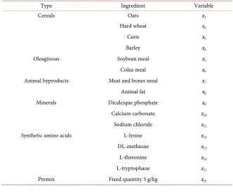
The ingredients and their corresponding variables are described in Table 1.

Table 2 contains the entire model together with the values of the technical coefficients of the model.

5.4. Software

The algorithm was programmed in MATLAB, which includes in its standard library the linear program solver called Linprog. This software can use the simplex method or an interior point method.

5.5. Two Criteria Models and Results

[image:12.595.207.540.461.736.2]

At first we analyse the relation between the cost of the diet and the two different excretions (nitrogen and phosphorus). As a curiosity, we also consider the interactions between the two kind of excretions: nitrogen and phosphorus.

Table 1. List of available ingredients.

Type Ingredient Variable

Cereals Oats x1

Hard wheat x2

Corn x3

Barley x4

Oleaginous Soybean meal x5

Colza meal x6

Animal byproducts Meat and bones meal x7

Animal fat x8

Minerals Dicalcique phosphate x9

Calcium carbonate x10

Sodium chloride x11

Synthetic amino acids L-lysine x12

DL-methione x13

L-threonine x14

L-tryptophane x15

(13)

(14)

5.5.1. Cost and Excretions

We have considered two separate bicriteria models. We look for least cost diets while taking into account the nitrogen excretion for the first model and the phosphorus excretion for the second model. For each of these two bicriteria problems, the Pareto curve indicates the diet cost increase caused by an excretion decrease.

While considering the nitrogen excretion, the problem is :

( )

1

2 ,

min min subject to

.

pr c pr

z cx

z q x

P

x = 

 ₌

  

 _∈

[image:14.595.301.444.178.236.2] [image:14.595.205.538.467.734.2]

 

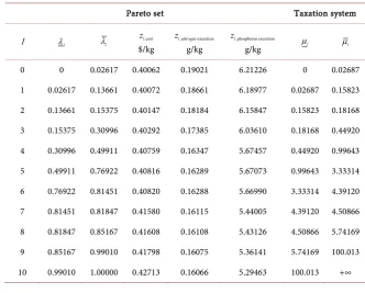
Table 3 presents the set of efficient extreme points of the Pareto set in the criterion space, and the Pareto curve is sketched in Figure 1. For this problem, the algorithm detects L=10_{segments and 11 efficient extreme points}

(

,1, ,2

)

(

,cost, ,nitrogen excretion

)

l l l l l

Q = z z = z z

for l=0, ,_ L=10_{. A total of 22 calls to the linear program solver was required}

(the predicted maximum is 2L+ =3 23_).

From its associated weighted-sum model given by

( )

(

,

)

(

) (

) ( )

1 2

( ) (

)

min ; 1 1

subject to

,

pr

c pr

z x z x z x c q x

P

x

λ λ λ λ λ

λ

 = − + =_ − + _ 



 _∈

 

Table 3. Efficient extreme points in the criterion space _2_{and the corresponding taxes}

for

(

P c pr

(

,

)

. and the corresponding taxes.

Pareto set Taxation system

l λl λl l,cost

z

$/kg

,nitrogen excretion

l

z

g/kg

,phosphorus excretion

l

z

(15)

[image:15.595.242.508.70.277.2]

Figure 1. Pareto curve: nitrogen excretion vs diet cost.

we get the following expression for its value function ϕ λ

( )

, defined for

[ ]

0,1

λ∈ , by

( )

min

{

z x

( )

; |x

}

(

1

)

zl,cost zl,nitrogen excretion

ϕ λ

=

λ

∈ = −

λ

+

λ

defined for

λ

∈ 

λ λ

l, l, and l=0, , L=10. So this expression depends on

the interval 

λ λ

l, l in which λ is.

For the parametric model given by

( )

(

,

)

(

)

1

( )

2

( )

(

)

min ;

subject to

,

ph

c pr

z x z x z x c q x

P

x

µ µ µ

µ

 = + = +

 

 _∈







we get the following expression for its value function ϕ µ

( )

defined for

[

0,

)

µ∈ +∞ _by

( )

min

{

z x

(

; |

)

x

}

zl,cost zl,nitrogen excretion

ϕ µ

 = 

µ

∈ = +

µ

defined for

µ

∈ 

µ µ

the interval 

µ µ

l, l in which µ is.

So we see that for any tax value in 

µ µ

l, l we will always have the same

expression for the value function ϕ µ

( )

, or the same behavior given by the efficient extreme point Ql=

(

zl,cost,zl,nitrogen excretion

)

, and the change in the

behavior will happend only when the taxation level µ_{passes through the}

extremities µl or µl of this interval

A similar analysis holds for the second bicriteria problem with phosphorus excretion. Indeed, for the phosphorus excretion problem, the model is:

( )

1

3 ,

min min subject to

.

ph c ph

z cx

z q x

P

x = 

 ₌

  

 _∈

(16)

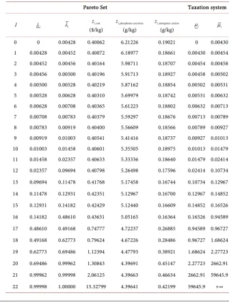
DOI: 10.4236/ajor.2018.85019 338 American Journal of Operations Research Table 4 presents the efficient extreme points in the criterion space while the Pareto curve is sketched in Figure 2. For this problem, the algorithm detects

22

L= _{segments and 23 extreme points}

(

,1, ,3

)

(

,cost, ,phosphorus excretion

)

l l l l l

Q = z z = z z

for l=0, , L=22. A total of 45 calls to the linear program solver was required (the predicted maximum is 2L+ =3 47).

From its associated weighted-sum model given by

( )

(

,

)

(

) (

) ( )

1 3

( ) (

)

min ; = 1 1

subject to ,

ph

c ph

z x z x z x c q x

P

x

λ λ λ λ λ

λ

 − + =_ − + _ 



 _∈

[image:16.595.201.537.297.739.2]

 

Table 4. Efficient extreme points in the criterion space _2_for

(

_{P c ph}

(

_,

)

_{, and the}

corresponding taxes.

Pareto Set Taxation system

l λl λl

,cost

l

z

($/kg)

l

z

(g/kg)

,nitrogenex cretion

l

z

(g/kg) µl µl

(17)

[image:17.595.231.518.61.297.2]

Figure 2. Pareto curve: phosphorus excretion vs diet cost.

we get the following expression for its value function ϕ λ

( )

_{defined for}

[ ]

0,1

λ∈ by

( )

min

{

z x

( )

; |x

}

(

1

)

zl,cost zl,phosphorus excretion

ϕ λ

=

λ

∈ = −

λ

+

λ

defined for

λ

∈ 

λ λ

the interval 

λ λ

l, l in which λ is.

For the parametric model given by

( )

(

,

)

(

)

1

( )

3

( )

(

)

min ;

subject to

,

ph

c ph

z x z x z x c q x

P

x

µ µ µ

µ

 = + = +

 

 _∈







we get the following expression for its value function ϕ µ

( )

defined for

[

0,

)

µ∈ +∞ _by

( )

min

{

z x

(

; |

)

x

}

zl,cost zl,phosphorus excretion

ϕ µ

 = 

µ

∈ = +

µ

defined for for

µ

∈ 

µ µ

l, l, and l=0, , L=22. So this expression depends

on the interval 

µ µ

l, l in which µ is.

So we see that for any tax value in 

µ µ

l, l we will always have the same

expression for the value function ϕ µ

( )

, or the same behavior given by the efficient extreme point Ql =

(

zl,cost,zl,phosphorus excretion

)

, and the change in the

behavior will happend only when the taxation level µ_{passes through the}

extremities µl or µl of this interval.

These problems of taxation are nice examples of abrupt (discrete) changes in behavior depending on the level of taxation of one criterion.

5.5.2. The Two Kinds of Excretion as Criteria

(18)

the two kinds of excretions are considered. This bicriteria problem is given by

(

)

2

3 ,

min min subject to

.

pr

ph pr ph

z q x

P

x = 

 ₌

  

 _∈

[image:18.595.300.445.93.150.2] [image:18.595.230.518.284.516.2]

 

Table 5 presents the set of efficient extreme points of the Pareto set in the criteria space. Its corresponding Pareto curve is sketched in Figure 3. This table shows the opposite effect of trying to reduce simultaneously both excretions. Minimizing one excretion leads to an increse in the other excretion. For this problem, the algorithm detects L=5_{segments and 6 extreme points. A total of}

12 calls to the linear program solver was required (the predicted maximum is

2L+ =3 13_).

For each l=0, ,5 , the value function is

Figure 3. Pareto curve: phosphorus excretion vs nitrogen excretion.

Table 5. Efficient extreme points in the criterion space _2_for _2_pour

(

_{P pr ph}

₍

_,

₎

)

_.

Pareto set

l λl λl l,nitrogen excretion

z

g/kg

l

z

g/kg

,cost

l

z

[image:18.595.209.538.573.734.2]

(19)

( ) (

1

)

zl,nitrogen excretion zl,phosphorus excretion

ϕ λ = −λ +λ

for

λ

∈ 

λ λ

l, l. For all value of the parameter λ in the interval 

λ λ

l, l we

will have the same expression for the value functionn ϕ λ

( )

or the same behavior

(

zl,nitrogen excretion,zl,phosphorus excretion

)

and a change in the behavior will

happend for values of the parameter λ_{corresponding to the extremities}λ_l

ou λl of this interval.

Let us observe that the last line of Table 3 (l=10_{) corresponds to the first}

line of Table 5 (l=0) and the last line of Table 4 (l=22) corresponds to the last line of Table 5 (l=5_).

6. Conclusion

In this paper we have considered bicriteria linear programming problems and have presented an elementary and efficient algorithm to compute the Pareto set in the criterion space. We have illustrated the method on a real important application. This application also suggests that it could be interresting to extend the method to three-criteria problems. Moreover it could be interesting to compare our method to other methods to find the Pareto set in the criterion space, but it is out of the scope of this paper and could be a nice subject for a future research.

Acknowledgements

This work has been supported in part by the Natural Sciences and Engineering Research Council of Canada and by the canadian corporation Swine Innovation Porc.

Conflicts of Interest

The authors declare no conflicts of interest regarding the publication of this pa-per.

References

[1] Dubeau, F., Julien, P.-O. and Pomar, C. (2011) Formulating Diets for Growing Pigs: Economic and Environmental Considerations. AnnalsofOperationsResearch, 190, 239-269. https://doi.org/10.1007/s10479-009-0633-1

[2] Adulbhan, P. and Tabucanon, M.T. (1977) Bicriterion Linear Programming. Com-puters&OperationsResearch, 4, 147-153.

https://doi.org/10.1016/0305-0548(77)90036-3

[3] Benson, H.P. (1979) Vector Maximization with Two Objective Functions. Journalof OptimizationTheoryandApplications, 28, 253-258.

https://doi.org/10.1007/BF00933245

[4] Cohon, J.L., Church, R.L. and Sheer, D.P. (1979) Generating Multiobjective Trade-Offs. WaterResourcesResearch, 15, 1001-1010.

https://doi.org/10.1029/WR015i005p01001

(20)

DOI: 10.4236/ajor.2018.85019 342 American Journal of Operations Research 301-307. https://doi.org/10.1007/BF00933233

[6] Geoffrion, A.M. (1967) Solving Bicriterion Mathematical Programs. Operations Research, 15, 39-54. https://doi.org/10.1287/opre.15.1.39

[7] Kiziltan, G. and Yucaoglu, E. (1982) An Algorithm for Bicriterion Linear Program-ming. EuropeanJournalofOperationlResearch, 10, 406-411.

https://doi.org/10.1016/0377-2217(82)90091-1

[8] Prasad, S.Y. and Karwan, M.H. (1992) A Note on Solving Bicriteria Linear Pro-gramming Problems Using Single Criteria Software. Computers&Operations Re-search, 19, 169-173. https://doi.org/10.1016/0305-0548(92)90090-R

[9] Sadagan, S. and Ravindran, A. (1982) Interactive Solution of Bicriteria Mathemati-cal Programs. NavalResearchLogisticsQuarterly, 29, 443-459.

https://doi.org/10.1002/nav.3800290307

[10] Walker, J. (1978) An Interactive Method as an Aid in Solving Bicriteria Mathemati-cal Programming Problems. Journal of the Operational Research Society, 29, 915-922. https://doi.org/10.1057/jors.1978.195

[11] Steuer, R.E. (1986) Multiple Criteria Optimization. Wiley, New York.

[12] Dubeau, F. and Kadri, A. (2012) Computation and Visualization of the Pareto Set in the Criterion Space for the Bicriteria Linear Programming Problem. International JournalofMathematicsandComputation, 15, 1-15.

[13] Benson, H.P. (1997) Generating the Efficient Outcome Set in Multiple Objective Linear Programs: The Bi-Criteria Case. ActaMathematicaVietnamica, 22, 29-51. [14] Bertsimas, D. and Tsitsiklis, J.N. (1997) Introduction to Linear Optimization.

Athenas Scientific and Dynamic Ideas, Belmont.

[15] Murty, K.G. (1983) Linear Programming. Wiley, New York.

[16] Chvatal, V. (1983) Linear Programming. W.H. Freeman and Company, New York. [17] Ferris, M.C., Mangasarian, O.L. and Wright, S.J. (2007) Linear Programming with

MATLAB, MPS-SIAM Series on Optimization, Philadelphia.

[18] Stigler, G.J. (1945) The Cost of Subsistance. Journal of Farm Economics, 27, 303-314.https://doi.org/10.2307/1231810

[19] Dantzig, G.B. (1963) Linear Programming and Extensions. Princeton Press, Prince-ton.

[20] Dantzig, G.B. (1990) The Diet Problem. Interfaces, 20, 43-47.

https://doi.org/10.1287/inte.20.4.43