FOR HIGH-RESOLUTION IONOSPHERIC SOUNDING
A thesis presented for the degree of Doctor of Philosophy in Physics in the University of Canterbury,
Christchurch, New Zealand.
by
S.H. Krenek :::::
CHAPTER 1: 1.1 1.2 1.3
CHAPTER 2: 2.1 2.2 2.3 2.4 2.5 2.6 2.7
INTRODUCTION 1
Ionospheric Observation Radars 1
The Development of Pulse Compression 2
Scope of This Work 5
MATHEMATICAL FOUNDATION OF PULSE COMPRESSION 7
Introduction 7
The Linear FM Expanded Pulse 7
Optimum Signal Processing and the Matched 13 Filter
Processing the Linear FM Signal 17
Range Sidelobe Reduction 20
Effects of Moving Targets 24
Summary 25
CHAPTER 3: DESIGN GOALS FOR A PULSE COMPRESSION RADAR
AT BIRDLINGS FLAT 26
26 28 3.1
3.2
CHAPTER 4: 4.1 4.2 4.3 4.4 4.5 4.6
A Brief History of Birdlings Flat Choice of System Parameters
DEVELOPMENT OF THE SIGNAL PROCESSING FILTER Introduction
Mathematical Analysis of the Proposed Filter Realisation of the Processing Filter
Application to Real Targets
5.1 5.2
Introduction
The Mathematics of Discrete Phase Modulation 5.3 Implementation of the Discrete Phase Modulator
Technique 5.4
5.5 5.6
5.7
Frequency Content of a Discrete Phase Modulated Chirp Pulse
Choice of Signal Parameters Practical Considerations
5.6.1 The Discrete Phase Modulator
5.6.2 The Modulation Command Controller 5.6.3 Control
Detailed Circuitry
5.7.1 General Considerations
59 61
67
72 75 80 80 81 86 86 86 5.7.2 The Discrete Phase Modulator Circuit 87 5.7.3 Modulation Command Controller Circuitry 89 5.7.4 Control Circuitry
5.7.5 Timing Considerations 5.8 Construction
5.9 Testing the Generator 5.10 Summary
CHAPTER 6: TRANSMITTER
CHAPTER 7: TRANSMITTING ARRAY
7.1 Theoretical Development 7.2 Practical Details
92 95 96 97 102
103
8.2 Circuit Descriptions 138
8.3 Construction 145
8.4 Bench Tests 145
8.5 Field Tests 148
8.6 Receiving Antennas 149
CHAPTER 9: SIGNAL PROCESSING SOFTWARE 150
9.1 Introduction 150
9.2 Computer Interfaces 151
9.3 Evaluation of the Filter Coefficients 152
9.4 Processing the Radar Returns 156
CHAPTER 10: SYSTEM EVALUATION 10.1 Hardware
10.2 10.3 10.4
Signal Processing
Performance with Ionospheric Returns General Comments
CHAPTER 11: CONCLUSION
APPENDIX: A.l A. 2
A. 3
A. 4 A.5
REFERENCES
ANCILLARY ELECTRONIC EQUIPMENT General
Frequency Converter
Mode Control and Line Driver Remote Pulse Width Control Transmitter Gating Control
ACKNOWLEDGE~1ENT S
160 160 164 168 178
180
183 183 184 186 188 190
195
Figure
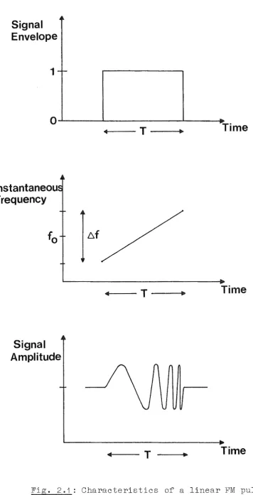
2.1 Characteristics of a linear FM pulse
2.2 Amplitude spectra for chirp pulses of various time-bandwidth products
2.3 Linear FM matched filter output envelopes (6f normalised to unity)
2.4 Effect of frequency weighting on the matched filter output
4.1 Effect of baseband mixing on signal spectrum 4.2 Baseband mixing technique
4.3 Block diagram of signal processing method 4.4 Effect of baseband mixing on filter output 4.5 Simulated processing of a single chirp pulse 4.6 Two chirp pulses 10 ~sec apart
4.7 Signal contaminated by Gaussian noise 4.8 Signal with offset in one channel 4.9 Output from truncated chirp pulse
4.10 Processing of a simulated ionospheric return
5.1 Relationship between continuous, sampled, and
5.2 5.3 5.4
quantised functions
Relationship between ~(t}, ~q(n} and qn Discrete phase modulation technique A square wave containing phase jumps
5.5 Frequency content of a square wave with constant phase jump rate
5.6 Some lines in the chirp spectrum
5.7 A method inserting phase jumps into a carrier
8
12
19
23
40 41 44 45 51 52 53 54 55 57
63 68 70 71
5.9 5.10 5.11 5.12 5.13 5.14
Modulation command controller principle Discrete phase modulator circuit
Simplified modulation command controller circuit Control circuitry
Waveforms of the sequential pulse generator outputs The chirp generator
5.15 Example of output from modulation command controller tests
84 88 90 93 94 98
100 5.16 Amplitude spectrum of chirp generator output 101
7.1 2.4 MHz narrowband transmitting array 108 7.2 Resistance (R) and Reactance (X) of a typical
half-7.3 7.4 7.5 7.6 7.7
wave dipole near resonance A cylindrical half-wave dipole A two-wire folded dipole
Impedances of a fictitious antenna A transmission line transformer
Configuration of optimum matching network for theoretical folded dipole
7.8 Array field patterns for 4-element broadside arrays
111 112 112 116 119
122
of different element spacings 124
7.9 Configuration of the proposed folded dipole 127 7.10 Similarity of susceptance functions for transmission
line stub and parallel tuned circuit 131 7.11 Feeder arrangement for each pair of dipoles 134 7.12 Magnitude of reflection coefficient at transmitter
[image:6.595.71.533.49.767.2]8.2 8.3 8.4 8.5 8.6 8.7
RF ampli circuit
Multiplier and low pass filter circuit Video ampli circuit
Loc~l oscillator configuration
RF amplifier frequency response Low pass filter characteristic
141 143 144 144 146 146
9.1 Effect of a linear added phase on a w~ighting function
and Fourier transform 155
10.1 Cosine and sine chirp signals mixed to baseband 163 10.2 Amplitude spectrum of the swept-frequency pulse 163 10.3 Compression filter output produced by a single chirp
10.4 10.5 10.6 10.7 10.8 10.9 pulse Compression approaching Ionospheric Ionospheric Ionospheric Ionospheric Ionospheric
filter output with the input signal noise level
returns, D- and E-regions returns, D- and E-regions returns, D- and E-regions returns, D- and E-regions returns, F-region
10.10 Ionospheric returns, F-region 10.11 Ionospheric returns, F-region
A.l A. 2 A. 3
A. 4
A. 5 A. 6
A phase locked loop
Frequency converter circuit
Mode control and line driver circuit
Block diagram of transmitter gating control RF line receiver circuit
Pulse width control circuitry
[image:7.595.72.540.101.815.2]ABSTRACT
A low frequency pulse compression radar system, capable of 0.75 km spatial resolution, has been developed. This system utilizes a linear frequency-modulated signal, and yields an
effective peak power enhancement of 14.5 dB, over a conventional radar of equivalent resolution.
The required instrumentation, as well as the development of the necessary signal processing software, are described in detail. It is shown that the resolution and peak power enhance-ment achieved by the system are consistent with those predicted by theory.
2.1 7.1
Properties of certain weighting functions
Terminal impedances for a theoretical folded dipole resonant at 2.4 MHz
7.2 Impedances appearing at input to transmission line transformer
7.3 Measured impedances at the driving point of a three-22
114
120
wire folded dipole 126
CHAPTER 1
INTRODUCTION
1.1 IONOSPHERIC OBSERVATION RADARS
Radar techniques have been widely used in the study of the ionosphere for many years, principally as a means of obtaining data relating to electron density profiles in the D-, E- and F-regions of the ionosphere. Conventional ionosondes presently in use employ pulsed radio-frequency emissions with peak powers typically in the tens of kilowatts, this power being sufficient to provide total re ection echoes having an adequate signal-to-noise ratio.
There are, however, certain applications which require the sounding pulses to contain substantially greater energy. One example concerns studies of the D-region, where the echo is caused by partial reflection processes (Gardiner and Pawsey, 1953) . The total energy contained in a pulse is clearly the product the peak power of the pulse, and its temporal length
(or 'pulse width'). This energy may therefore be increased by increasing either, or both, of these factors.
To increase the peak power output of a transmitter is
always expensive, and, in extreme instances, is not technically feasible. Further, the use of transmitters having very high peak powers can result in cross modulation effects which alter the structure of the ionosphere its f.
On the other hand, an increase in the width of the trans-mitted pulse is easily accomplished; however, the spatial
according to the relation
0
=
(L 1)where T is the pulse width
c is the speed of electromagnetic radiation.
Thus an increase in the pulse width effects a correspond-ing degradation in the spatial resolution of the radar system.
Radar studies of the ionosphere are conducted at a field station of the University of Canterbury, situated at Birdling's Flat, near Christchurch. Interest has been shown in investig-ating the fine structures of electron density irregularities which give rise to radar echoes from the ionospheric D-region. Such a study would require a radar system capable of a high resolution. Also, since D-region partial reflections are characteristically weak, the energy contained in the sounding pulses should be maximised. These two requirements are clearly in conflict, and a project was initiated to resolve this dilemma.
1.2 THE DEVELOPMENT OF PULSE COMPRESSION
The conflict between high pulse-energy and good resolving power is by no means restricted to ionospheric sounding radars, and in fact was first investigated by engineers faced with the shortcomings of the military radars in use during World War 'II. It was well known that the bandwidth, ~f, of a pulsed radio-frequency signal was directly related to its pulse width, according to the Fourier relationship
~f 1
An inverse relationship thus exists between the resolving power and bandwidth of a radar signal, of the form
0
=
c2L'If ( 1. 3)
The key to the solution of the energy-versus-resolution dilemma lay in the realisation that i t is the bandwidth, and
not the pulse width, which fundamentally determines the potential resolving power of a signal. This fact was recognised indepen-dently by several workers serving on both sides of the war. In this regard, Hlittman (1940) was issued a German patent covering his work during the late 1930's. Sproule and Hughes (1948) were granted British patents, and later Dicke (1953) and Darlington
(1954) received American patents, all of these relating to work accomplished during the final years of the war.
The methods described in these patents all proposed the transmission of a wide pulse, the frequency of which was varied linearly throughout its duration. By virtue of its width, this 'linear frequency-modulated' pulse would contain a high energy. Moreover, i t seemed intuitively obvious that, as a consequence of the wide bandwidth over which the frequency was 'swept', good resolving power should be attainable with this signal.
There are two instances which are known to occur in nature which lend support to this hypothesis. The following is para-phrased from a report on the ultrasonic emissions of bats
(Griffin, 1950)
"The bat emits a series of ultrasonic pulses about two milliseconds in width, at a repetition frequency of 10 to 20 Hz. The most striking feature is that the frequency of the pulse is not constant, but
the length of a two millisecond pulse in air is about 70 em, suggesting that the bat must make use of the frequency modulation inherent in the pulse to indicate target distance, since bats have no
locating food and obstacles by accoustic means even at
5 em."
In his book "The Mind the Dolphin" (Lilly, 1967) the author describes the complex sonar of TuPsiops tPuncatus~ a species of dolphin possessing a level of intelligence approaching, if not surpassing that of Homo sapiens. Experiments with these animals indicate that they employ a number of different sonar signals, one in particular consisting of a pulse about 0.3 seconds long, rising in frequency from about 5 KHz to 25 KHz. The dolphin is observed to use this signal for observing close objects, making the transmitted pulse long enough to overlap with the received echoes. Lilly suggests that such a situation would produce beat notes a constant frequency between the transmitted and
received signals, enabling the dolphin to make an accurate determination of target range. Though the transmitted pulse is hundreds of meters in length, resolutions as low as 7 em would be obtainable using this technique.
Early workers in the field intended that the latent high resolving power inherent in the linear frequency-modulated pulse be exploited by passing the received radar echo through a
A complete description of the theory of pulse compression was originally published in a comprehensive paper by Klauder et
al. (1960). Included in this report were treatments of both optimum ('matched filter') and practical means for compressing the received radar echoes. Klauder also introduced the
appellation 'chirp' to describe a linear frequency-modulated pulse, and this terminology will be adopted throughout this thesis.
1.3 SCOPE OF THIS WORK
Pulse compression techniques have previously been employed to enhance ionospheric observation radars. A comprehensive
study (Wipperman, 1967) established the feasibility of utilising pulse compression techniques to enhance radars used in ionos-pheric work. Barry and Fenwick (1965), and more recently
Rinnert et al. (1976) used a pulse compression method enabling the use of low transmitter powers for D-region studies, while as early as 1954, Gnanalingum (1954) used what is effectively a pulse compression system, later adopted by Titheridge (1962).
It seems clear, therefore, that the use of pulse compression would be a viable means of overcoming the
energy-versus-resolution problems associated with a study of the fine
of the available resources at the Birdling's Flat field station. Part of the design philosophy adopted was that the system be,
as far as possible, compatible with the instrumentation already existing at that site.
A major achievement during the course of this work was the design of a highly-linear frequency-modulated pulse generator, which utilized only digital circuit elements. A novel approach to the implementation of the compression filter was also
developed, offering distinct advantages over previously reported systems.
In the next chapter a rigorous mathematical treatment of pulse compression is presented. This is followed by a brief description of the field station at Birdling's Flat, and a statement of the design goals for the proposed system. The design and construction of the instrumentation and software required to implement the system are then reported in detail. Finally, an evaluation of the completed system is given,
CHAPTER 2
MATHEMATICAL FOUNDATION OF PULSE COMPRESSION
2.1 INTRODUCTION
This chapter contains the formal mathematics of the pulse compression method. Underlying the development which follows is the premise that potential resolving power of a radar signal is dependent solely on the bandwidth of the transmitted signal (and thus independent of its pulse width).
The signal considered during the development is the linear frequency-modulated, or 'chirp' pulse, introduced in the
previous chapter. It should, however, be recognised that linear frequ-ency nodulation is only one a number of modulation schemes capable of producing a pulse of the required bandwidth. The signal is also assumed to have a rectangular amplitude envelope, since this maximises the energy contained in each pulse.
The treatment of pu!se compression first considers the frequency content of the linear FM pulse (often cal the
'expanded' pulse, to distinguish i t from the 'compressed'
pulse appearing after signal processing) . From this frequency content is derived the form of the optimum signal processing
lter. Finally, an expression for the signal at the output of this (i.e. the compressed pulse) is developed.
2.2 THE LINEAR FM EXPANDED PULSE
The expanded pulse is shown diagrammatically in Fig. 2.1. The instantaneous frequency of the pulse is centred upon f
Signal
Envelope
1-r-o~----~---~---.
Time
lnstantaneou
Frequency
Signal
Amplitude
+ - - - T - - +
+ta~--T---.
.,..,. _ _ T
Time
Time
[image:17.595.91.448.87.785.2]f
0 - t:,f/2 to f0 + t:,f/2. The mathematical expression for such a signal is
e(t)
=
rect(~)
exp{2ni(f0t +
k~
2)}
where f
0 is the centre frequency of the signal T is the pulse width in seconds
k is the rate of frequency modulation.
The function rect(z) (Woodward, 1953) is defined as
rect(z)
=
1 if lzJ < !-zrect(z)
=
0 if lzJ > !-z( 2 .1)
This function provides the signal with a rectangular envelope between t
=
-T/2 and t=
+T/2. The signal is arbitrarily chosen to have unit amplitude.As usual the actual signal is obtained by taking the real part of the complex expression given in equation (2.1). The phase, ¢, of e(t) is of course given by
=
( 2 • 2)and the instantaneous frequency, f., at any particular time is
1
found from
f,
1
=
=
( 2 • 3)Equation (2.3) shows that the signal contains the desired linear FM property, since during the T-second interval of the
kT kT
pulse, the frequency varies linearly from f
The frequency deviation ( or 'swept bandwidth'), 6f, of the signal is just the difference between these two limits, i.e.
6f
=
kT ( 2. 4)It is thus demonstrated that the signal e(t) possesses the characteristics shown in Fig. 2.1. However, since the signal is limited in time, the actual frequency content of each pulse will not be adequately specified by equation (2.3); a complete
description of the spectrum of the signal can only be obtained by Fourier analysis.
If A(f) denotes the Fourier transform of some arbitrary time function a(t), then the Fourier transform of equation (2.1) will be given by
E(f)
=
J:
00
e(t) exp{-2nift}dt
=
f
T/2 exp{2ni(f -f)t + kt }dt 2-T/2 o 2
( 2. 5)
It can be shown (Chin and Cook, 1959) that this integral has a solution
( 2 • 6)
where Z(u) is the complex Fresnel integral, defined as
Z(u)
=
C(u) + iS(u)=
f
u 2
=
,F¥]
=
( 2 • 8)The amplitude spectrum of e(t) is obtained by taking the absol-ute value of equation (2.6):
( 2 • 9)
Some further algebraic manipulations (Cook, 1960) of the Fresnel integral arguments yield the result
ul =
fz
[l
+2 (f-fol] ./':,.f
J
14
rl _ 2 (f-f 0)j
(2.10) u2 = 2L
f'::,fwhere D
=
T/':,. f .This quantity D is called the 'time-bandwidth product' of the signal. It is also variously known as the 'dispersion factor' or the 'compression ratio' of the system; the signific-ance of these alternate terminologies will become apparent later. The time-bandwidth product is the most important factor relat-ing to the performance of a pulse compression radar system.
Inspection of equations (2.10) and (2.9) yields the important result that the shape of the amplitude spectrum of e(t), when plotted against (f-f
0)/l':,.f, is dependent only on the time-bandwidth product, and not the absolute frequency deviation, /':,.f. Equation (2.9) has been evaluated for various values of D,
and the normalised results plotted in Fig. 2.2 (from Klauder et al., 1960). It can be seen that as the time-bandwidth
Spectrum
Amplitude
Spectrum
Amplitude
Spectrum
Amplitude
0=10
Frequency
0=60
Frequency
0=120
Frequency
[image:21.597.59.551.56.830.2]and more clearly contained in the frequency interval £
0±6£/2. However, i t has been calculated (Klauder et al., 1960) that even for values of D as low as ten/ ninety-five percent of the
spectral energy is contained within the band of interest. This completes the description of the linear FM expanded pulse, which is a suitable signal for emission by the trans-mitter of a pulse compression radar system. In the next
sections i t is shown how an echo received from a transmission of this nature may be 'compressed' in time by passing i t through a suitable filter.
2.3 OPTIMUM SIGNAL PROCESSING AND THE MATCHED FILTER
The received radar'return should be processed in such a manner as to maximise the information which can be extracted from it. It is not immediately obvious what philosophy must be pursued to achieve this goal. Woodward (1953) discusses several criteria for just which quantity should be maximised. Since the presence of noise is the major factor contributing to the degradation of signal quality, i t is usual, though not univer-sal, to attempt to maximise the signal-to-noise ratio of the radar return. Specifically, a processing filter will be desig-ned which maximises the ratio of peak signal .power to the mean noise power.
So far, only linear FM signals have been considered; for the following discussion, the treatment will be broadened to apply to any time function.
As before, the Fourier transform of an arbitrary time
network admittance function, Y(f). If i t is assumed that the noise contaminating the signal is Gaussian, the signal-to-noise ratio at the filter output may be expressed as (Klauder et al., 1960) :
s
N
=
IJY(f) .A(f) exp{2Tiiftm}dfl 2
f
I A (f) 12
df
f
I y (f) j2 df
where tm is the time at which the right hand side of the
( 2 .11)
equation is a maximum. t will, in general, be a function of m
both Y(f) and A(f).
Since the signal, A(f), is normally already specified, the problem reduces to finding a Y(f) which maximises equation
(2.11). This is a problem in the calculus of variations,
whose solution is summarised in the Schwartz inequality, which states that for two arbitrary functions, f(z) and g(z),
2
IJf(z)g(z)dzl
< 1 ( 2 • 12)
The equality holds only when f(z) is proportional to g*(z) (where the * operator indicates complex conjugation) .
Application of the inequality to equation (2.11) indicates that the maximum signal-to-noise ratio at the output of the filter occurs when
Y (f) a: A* (f) exp{ -2 TiiftrJ (2.13)
the matched filter for any time signal a(t) is defined by
y (f)
m A* (f) ( 2. 14)
where the constant of proportionality has been arbitrarily chosen to be unity.
It is important to realise that the preceeding development is valid irrespective of the signal configuration; any signal passed through its own matched filter maximises equation (2.11) to unity.
An expression for the output of a filter which is matched to its input signal will now be developed. The frequency
domain representation of the filter output is given by
A
0 (f)
=
Y m (f) .A. (f) lwhere A (f) is the spectrum of the output signal
0
A. (f) is the input signal spectrum. l
( 2 • 15)
This follows directly from the definition of the admittance function of a filter. Substituting equation (2.14) into equation (2.15) yields the important result:
or
A(f)
=
A.*(f).A(f)0 l
A (f)
=
0
2
JAi (f)
I .
( 2 .16)The corresponding time domain relationship follows from the well-known property of Fourier transforms: multiplication of two functions in the frequency domain is equivalent to con-volution in the time domain.
Hence
where y (t) is the impulse response of the filter and x is
m
the convolution operator, defined such that for two arbitrary functions, f(z) and g(z),
f(z) x g(z)
=
j_
roo
00
f(z-w)g(w)dw ( 2 • 18)
Taking the inverse Fourier transform of equation (2.14) leads to the relation
( 2 . 19)
Substituting equation (2.19) into equation (2.17) then gives the result
a (t)
=
a.* (-t) x a. (t)0 l l (2.20)
or (2.21)
Equations (2.16) and (2.21) describe the output from a matched filter in the frequency and time domains respectively, and each embodies a result of fundamental significance.
Equation (2.16) shows that the output signal from a matched filter is the Fourier transform of the power spectrum of the input signal. Equation (2.21) demonstrates that the filter
2.4 PROCESSING THE LINEAR FM SIGNAL
An expression for the output of a filter matched to a
linear FM pulse may now be developed. It will be recalled that this signal is described by
( 2. 1)
The form of the matched filter for this signal follows directly from the definition given in equation (2.14):
Y (f)
=
E* (f)m (2.22)
where E*(f) can be readily obtained from equation (2.6). Sub-stituting leads to
(2.23)
The output of this matched filter, e (t), may be obtained from
0
equation (2.21):
e ( t)
0
=
Jroo
-00 e.*(T-t) e. (T)dT l l=
J
oo T-t T . kT2 k(T-t) 2}
-oo
rect ( ' I ' ) rect (T) exp{ 2rrl (f0 t + - 2- - 2 dT ( 2. 24)
This integral is readily evaluated (Cook, 1961) to give
e ( t)
0 sin
2
rr (ktT-kt ) (2.25)
15
sinTI(~fltl
-~f
2t
2/D)
TI~fltl (2.26)
This term represents the amplitude envelope of the filter out-put. As before, D is the time-bandwidth product of the chirp pulse. Fig. 2.3 shows the shape of this envelope for various values of D. It can be seen, and indeed is obvious from inspection of (2.26) that this envelope approximates a sin x
X function, and that th approximation improves as D increases.
The shape of the envelope described by (2.26) is of paramount importance, for embodied in is the realization the aims of pulse compression. The llowing points should be noted:
a) The amplitude the output pulse has been increased by a factor of
10.
b) The width of the 'compressed' pulse, T, taken at the -3 dB points of the main lobe, is given approximately by
T
=
1 (2.27)The effective resolution achieved is thus dependent only on the bandwidth of the transmitted pulse. Further, the ratio of the expanded to the compressed pulse widths is given by
T
T T~f
=
D (2.28)The significance of describing D as the 'compression ratio' of the system now becomes apparent.
Response Amplitude
0=10
-10
-a.
-6 -4 -2
2
4
6
a
10
Time (Seconds)
Response Amp I itude
0=50
-10 -8 -6 -4 -2
0
2
4
6
8 10
Time (Seconds)
2.5 RANGE SIDELOBE SUPPRESSION
Consider again the envelope of the matched filter output, shown in Fig. 2.3. The major lobe, of course, represents the position of the radar echo; the minor lobes, since the X-axis is a time axis, occur before and after the main response, and accordingly are referred to as range sidelobes. For a true sin x .
funct1on, the closest of these have an amplitude of -13 X
dB relative to the main lobe. Clearly, in a multitarget en-vironment, or, as in the ionosphere, with a distributed target, there is a problem with data interpretation, when the sidelobes from a strong echo could easily mask the main lobe of an adjac-ent weaker echo. A number of methods have been used to reduce the amplitude of these sidelobes, all based upon tailoring the frequency response of the receiving system according to some particular "weighting function".
A weighting function is a function, defined over a finite sin x frequency range, possessing a Fourier transform with a
X like envelope. This envelope, however, differs from a sin x
X function in some important aspects:
a) It has vastly reduced sidelobe amplitudes (typically around -40 dB relative to the main lobe)
sin x b) The main lobe is somewhat broader than that of a
X function
c) The amplitude of the main lobe is about one dB less sin x .
than that of the funct1on. X
condition of lowest sidelobe levels for a given amount of main lobe broadening. The generalised cosine-power functions are given by the formula
w
(f)=
k + (1-k) (2.29)which represents a cosine-power function, centred about f0, sitting on a 'pedestal' of height k.
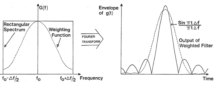
The means by which a weighting function effects a suppression of the range sidelobes is as follows. For the purposes of this discussion, i t will be assumed that the spectrum of the chirp signal is rectangular, i.e.
=
0 elsewhere. (2.30)The frequency-domain representation of the output of a filter matched to this signal may be obtained from equation (2.16):
E (f)
=
JE(f)\ 20
== 0 otherwise. (2.31)
The output signal will thus be a sinusoid of frequency f
0, with sin x
a -shaped envelope. If this output pulse is passed X
through a filter having an admittance function W(f) (where W(f) is some weighting function), then the output of this filter, E (f), will be given by
=
0 elsewhere ( 2. 32)The output of the filter in the time domain will thus be the Fourier transform of the weighting function. Note that the frequency range over which W{f) is defined must be such that i t encompasses the rectangular spectrum E(f) exactly. Also,
since W(f) is centred upon f
0, the output of the weighting fil-ter will be a sinusoid of frequency f
0, with an envelope dependent on W(f). Fig. 2.4 will help clarify this.
Note that the output pulse from the weighting filter is broader than the unweighted signal; the magnitude of this broadening is known as the 'pulse widening factor' of the weighting factor. The amplitude decrease of the weighted pulse is often called the 'mismatch loss' introduced by the weighting filter.
Some of the most commonly used weighting functions and their effects on the matched filter output pulse are presented in Table 2 .1.
Table 2 .1 Properties of certain weighting functions. Function
Dolph-Chebyshev Taylor approximation Generalised Cosine-power:
Hamming (k • 08, n = 2)
Hanning (k
=
O, n = 2)Peak Sidelobe Level (dB)
-40 -40
-42.8
-32.2
Pulse Widening Factor
1.35 1.4
1.47 1.62
Mismatch Loss(dB)
0
-1.2
-1.34
-l. 76
Rectangular/',..~
., ...
Spectrum ,/
~\Weighting
I ,../
\\~7tion
I '
,
I"
.-"""" I I I I I I I I,
' \ ' \ ' \ \ \ \ ~'
\'
'..
... ,_ FOURIERfo-~f/2
fo
f0
+~fj2
Frequency
I I I I I I I I I
,
I I I I I I I I I I I I I I \ \~Sin
1ft
6.f
\
.
-rrt~f
I I I \ \
\ Otitput of
\Weighted Filter
\
Time
Fig. 2.4: Effect of frequency ghting on the matched filter output.
N
[image:32.842.40.774.184.494.2](see Fig. 2.2). Failure to allow for this fact during the
design of a weighting filter results in considerable degradation of the attainable sidelobe levels, especially for low values of D (Klauder et al., 1960). This aspect is examined in more
detail in chapter 4.
2.6 EFFECTS OF MOVING TARGETS
The mathematical development has so far implicitly assumed negligible doppler shifting of the radar signal due to radial velocity of the target. A more general derivation (Cook, 1961) shows that this assumption is justified only if the doppler frequency, fd' is small compared to ~f, the 'swept bandwidth' of the chirp signal.
The doppler frequency may be obtained from the formula
=
where f
0 is the centre frequency of the signal vt is the radial velocity of the target
(2.33)
c is the velocity of electromagnetic radiation. Rearrangement leads to the inequality
(2.34)
2.7 SUMMARY
In this chapter i t has been demonstrated that the principle of pulse compression has a sound theoretical basis. The origin-al premise that the potentiorigin-al resolving power of a radar signorigin-al is dependent only on its bandwidth has been validated. Further, i t is shown that the compression process effects an increase in the peak power of each received pulse, the magnitude of which
i
CHAPTER 3
DESIGN GOALS FOR A PULSE COMPRESSION RADAR AT BIRDLING'S FLAT
3.1 A BRIEF HISTORY OF BIRDLINGB FLAT
Ionospheric research has been firmly established at Canter-bury University for some decades, most of the early practical work being carried out at the University's field station at Rolleston. By about 1961 however, the available ground space there was becoming severely limited, especially for the large transmitting and receiving arrays required for work at lower
frequencies. Accordingly, a search for a new site was conducted, and a lease eventually secured for the present field station at Birdling's Flat (location 172.7°E, 43.8°S; magnetic inclination,
22° to the vertical).
This area is well suited for use as an upper-atmosphere research installation for a number of reasons:
a) Situated on several square miles of flat land, i t offers almost unlimited space for large antenna arrays.
b) Since i t is located about 50 km from the city, man-made electrical noise is at a minimum.
c) It is a coastal site, a prerequisite for the use of atmospheric sounding rockets.
A grant from the U.S. National Science Foundation provided sufficient finance to install the initial equipment at the site. This included two 100 kw pulse transmitters, plus receiving and data recording equipment. All the instrumentation was
Early work at Birdling's Flat in~luded electron-density measurements using the Differential Absorption technique
(Gardiner and Pawsey, 1953). Data was recorded manually from measurements of the trace on a cathode ray tube displaying the ionospheric returns. This was a tedious process, and most workers in the field contributed something towards a more auto-mated data reduction system (Shearman, 1962; Manson, 1965;
Austin, 1966). Studies of ionospheric winds were also conducted during the first few years of operation at Birdling's Flat.
Dedicated hardware was utilized to produce a one-bit correlation of the signals from three antennae, the data being output to a paper tape punch (Fraser, 1965, 1968).
The instrumentation at the field station was substantially upgraded in 1972 with the purchase of a DEC PDP8e minicomputer. This initiated important progress in two distinct areas.
Firstly, the field station could be placed entirely under soft-ware control, enabling routine data-collecting experiments to be performed in the absence of personnel. Secondly, full data processing could be undertaken in the field, with the conse-quent advantages of immediate evaluation of equipment perfor-mance and experimental techniques. An excellent description of on-line control of ionospheric sounding experiments may be
found in Fraser (1973) .
The only major change in the station hardware since 1972 has been the replacement of electron tube-based equipment with semiconductor units. With the exception of the transmitters, there is presently no valve-operated equipment in use at
3.2 CHOICE OF SYSTEM PARAMETERS
The selection of the parameters for the proposed pulse compression radar system is dependent to some extent on the
nature of the experimental work for which the system is intended. It will be recalled (chapter 1) that this project was initiated principally to assist an anticipated study of the fine structures present in the D-region electron densities. Any decision
regarding the resolving power of the proposed system must therefore be made with due regard to the physical size of the electron density irregularities present in the ionosphere.
It was assumed (von Biel, 1975) that little structure exists in the D-region of characteristic size less than about 1 km; accordingly, i t was decided to attempt a system resolving power of 0.75 km. A signal bandwidth of 200 kHz is required to achieve this resolution (see equation (1.3)). For a convent-ional radar, this is equivalent to a pulse width of 5 micro-seconds. The transmitting licence for Birdling's Flat requires the signal frequency to be centred on 2.4 MHz; the chirp signal must therefore vary in frequency between 2.3 and 2.5 MHz.
The direction of frequency modulation is arbitrarily chosen to be positive.
unrealistic demands on the linearity and dynamic range of the receiving and processing system. The restriction is thus created that the transmitted pulse must have ceased before radar returns from the closest target of interest arrive. I t can safely be assumed that ionospheric returns will not be received from below about 60 km; this height is equivalent to an echo time of 400 ~sec. This figure hence provides an upper limit for the transmitted pulse width.
There are, however, technical factors which also govern the range of permissible pulse widths. For example, the output tubes in the transmitter will have a certain maximum period of continuous operation, which, i f exceeded, will result in rapid deterioration of the tube cathodes. For the transmitter at Birdling's Flat, this constraint is far more severe than that discussed in the previous paragraph; consultations with the designer of the transmitter indicated that i t would be most unwise to attempt a pulse width greater than 150 ~sec. This value was therefore adopted.
The following list summarises the proposed parameters for the pulse compression radar system.
Type of signal= linear FM ('chirp') Swept bandwidth, b. t
=
200 kHzCentre frequency
=
2.4 MHzExpanded pulsewidth, T
=
150 ~secCompression ratio, Tb.f
=
30.The actual resolution achieved by the system is expected to be somewhat larger than 0.75 km, due to 'main lobe
CHAPTER 4
DEVELOPMENT OF THE SIGNAL PROCESSING·FILTER
4.1 INTRODUCTION
In general, the radar return from a linear FM pulse trans-mission consists of a number of overlapping expanded pulses, each with some particular amplitude and phase. This return requires some form of processing in order that the resolution potential inherent in the signal may fully real It was shown in chapter 2 that the optimum processing network which achieves this is a matched filter. Although the theory of
matched filtering was fully understood early in the development of pulse compression, i t was not until recently that the tech-nology was of a sufficiently high standard to permit realisation of a true matched filter. Previously, workers were forced to substitute various approximations.
One of the most common early implementations of the
compression filter propagated the expanded pulse down an ultra-sonic delay line, which exhibited a linear time delay-versus-frequency characteristic (Fitch, 1960; Wipperman, 1967). Such a device, if the parameters were chosen correctly, presented a filter function to the incoming signal of the form
( 4 .1)
It can be seen that this will approximate the matched filter function, given in equation (2.23), reasonably well if the term
[Z* (u
a linear FM pulse is similar to the matched filter response, with the exceptions that
Sin X a) The envelope of the output pulse is a true X function,
b) The frequency inside this envelope is linearly modulated at the same rate as the input signal, but in the opposite
direction.
It is most instructive to consider this example of the dispersive delay line, as i t can give a clear intuitive picture of how a compression filter operates. Since the velocity of propagation in the line is a linear function of frequency, i t may be readily appreciated that the trailing edge of the ex-panded pulse can be made to propagate faster than the leading edge, causing the two to reach some point in the line simultan-eously. A compression of the pulse is thus effected.
Other devices are known to exhibit dispersive delay
characteristics, for example lumped constant bridged T networks. If a number of these all-pass time delay equalisers are design-ed for different delays and then cascaddesign-ed, the resulting filter can be made to exhibit a linear delay-versus-frequency charac-teristic over a restricted range with reasonable accuracy
(O'Meara, 1959; Brandon, 1965).
performing the convolution (Cutronoa et al., 1960; Reich and Slobodin, 1961; Slobodin, 1963) .
Another method first introduced in 1971 propagated a chirp signal and its time inverse as surface acoustic waves from
opposite ends of a Lithium Niobate plate, to achieve a convol-ution of the two directly. In initial experiments, bandwidths of up to 400 MHz were demonstrated (Bongianni, 1971; Grasse, 1971).
The discovery of the Fast Fourier Transform (Cooley and Tukey, 1965; Brigham and Morrow, 1967) initiated a new approach to signal processing. Techniques were developed by which
filters could be implemented arithmetically, using digital computers. Two distinctly different approaches are in general use:
a) Processing in the time domain with recursive or non-recursive digital filters (Rader and Gold, 1967; Helms, 1968; Echard and Boorstyn, 1972; Gray and Nathanson, 1971).
b) Transforming a time series into the frequency domain with a Fast Fourier Transform (FFT), multiplying the spectrum by the filter function, and transforming the product back into the time domain (Hart and Sheats, 1971; Halpern and Perry, 1971) .
The second method is more useful for complicated filter functions, since the filter can be implemented as soon as its frequency response (whatever form i t may take) is known. This aspect will be dealt with in greater detail later in this
In the past, many processing methods which were perfectly valid mathematically were unuseablebecause of technological
limitations. However, with the availability of the computation-al filters just described, i t may be assumed that such
restrictions no longer apply.
4. 2 MATHEriJATICAL ANALYSTS OF THE PROPOSED FILTER
The mathematical treatment of range sidelobe suppression (section 2.5) clearly indicated that the optimum form of the out-put from a pulse compression signal processing network was the Fourier transform of the chosen weighting function. For a
simple weighting filter, this situation only occurs if its input has a rectangular spectrum. Since the spectrum of the matched filter output is not rectangular, use of a simple weighting filter will cause some signal degradation, which is manifested as an increase in the sidelobe levels of the filter output. Cook and Paolillo (1964) have calculated that the magnitude of this increase is about 10 dB; clearly, this results in unaccep-tably large range sidelobes. Even so, the presence of Fresnel spectral ripples is often neglected in the design of a pulse compression signal processing filter. It was, however, determin-ed that this would not be the case in the present work.
The frequency domain output of a filter matched to the chirp waveform is by definition
( 4 • 2)
where E(f) is the spectrum of the input signal, taken to be a chirp pulse centred aroung t
=
0The matched filter is defined by
y (f)
m E* (f) (2.22)
which leads to
E
0 (f)
=
E (f) •E* (f) ( 4. 3)Introducing the signal E
0 (f) into a weighting filter gives
E (f)
ow E0 (f) ·W (f)
=
E(f)·E*(f)•W(f) (4.4)where W(f) is a weighting function and E (f) represents the output
OW the weighting lter.
The width and position of the weighting function is
chosen, of course, so that i t encompasses the usable portion of the chirp spectrum (see Fig. 2.4). It will be recalled that optimum output from the weighting filter is predicated upon the fact that its input has a rectangular spectrum. This may be ensured by preceding the weighting filter with a filter V(f), which is specified such that when applied to the matched
lter output, i t transforms the signal into one with a
rectangular spectrum of similar bandwidth. Let W' (f) denote the filter found by cascading V(f) and W(f). That is,
W' (f)
=
V(f) .W(f) ( 4. 5)E ow , (f) = E (f) . Y m ( f) .
v (
f) . W ( f)= E(f).E*(f).V(f).W(f) ( 4 • 6)
Inspection of equation (4.6) shows that if V(f) is to perform its specified function, i t must be of the form
v
(f)=
E(f) .E*(f) 1
=
0 elsewhere ( 4. 7)The output of the composite filter then becomes simply
E , ( f ) = W(f)
ow ( 4 • 8)
as desired.
Inspection of equations (4.5) and (4.7) shows that optimum signal processing will be achieved if the simple weighting fil-ter W(f) is replaced by a filfil-ter W' {f), given by
W' (f)
=
E(f).E*(f)
w
(f)( 4 • 9)
If this is the case, the time domain output of the
processing filter will be the Fourier transform of the weight-ing function.
Let Yc(f) be defined as the network admittance function of a complete signal processing filter, formed by cascading Ym(f) and W' (f).
Then, by definition
E I (f)
=
E(f) .Y (f)Comparing this with equation (4.8) leads to the fundamentally important result that
E(f).Y (f)
=
W(f) cor y (f)
c
=
w
(f)E (f) ( 4 • 11)
Equation (4.11) gives an expression for the admittance function of a complete signal processing filter, Y (f), which compresses c the chirp signal, compensates for Fresnel ripples in its spec-truro, and applies frequency weighting to reduce the sidelobes. This filter function may be readily obtained knowing only the spectrum of the chirp signal, and form of the chosen weighting function.
4.3 REALISATION OF THE PROCESSING FILTER
This section describes how the proposed signal processing filter, Y (f), is physically realised. Earlier in this chapter,
c
i t was indicated that given the availability of digital comput-ing power, a mathematical rather than an electronic implementat-ion would be most appropriate.
Time domain digital filtering was studied carefully as a possible means of realising the filter. This technique, though storage requirements are modest, often necessitates large
These disadvantages do not apply to frequency domain filtering, though this method does require considerably more computer storage. However, the PDP8 at Birdling's Flat was
equipped with a large memory (16K words), and since an efficient FFT routine was available (Rothman, 1968) i t seemed clear that implementing the processing filter in the frequency domain would be the superior approach.
The operation of the Fast Fourier Transform is well known and has been reported widely in the literature (Cooley and
Tukey, 1965; Brigham and Morrow, 1967; Brigham, 1974), and will not be described here. It should, however, be understood that the transform operates on a sequence of time samples (usually some power of two in number) and returns an equal number of coefficients, representing the magnitudes of the frequency com-ponents present in that sequence.
Implementation of a filter in the frequency domain requires first that the input signal be sampled at fixed intervals, and that these samples be converted to digital form. These digital samples are then transformed into the frequency domain by an FFT. The resulting spectrum is multiplied point by point by the filter function, and the product transformed back into the time domain. Two points concerning this process should be noted.
a) The FFT coefficients in both the time and frequency
domains are in general complex (representing amplitude and phase), as is the filter function.
A discrete function is formed as a result of sampling a continuous function. It may be written in the form a(j), where
j may have only integral values. For example, a sinusoidal signal of frequency f
0, expressed in continuous form by
g(t)
=
(4.12)would be described after sampling by
g(j) = (4.13)
where j
=
0,1,2, ...and t is the sampling interval. s
A selection of a finite number of these samples, say those with 0 ~ j ~ 255, would provide a set of 256 complex amplitudes
which would be in a suitable form to be processed by a discrete Fourier transform.
The actual sampling is performed by an analogue-to-digital converter, which converts an electrical voltage into an
equivalent digital word which can be read by the computer. Care must be exercised in the selection of the sampling frequency, since a series can only represent a continuous function accurately if there are at least two samples per period of the highest frequency present in that function. An inadequate sampling rate will result in the well-known phenomena of aliasing and spectral foldover (Brigham, 1974; Blackman and Tukey, 1958).
technique keeps the frequencies present in a signal as low as possible by mixing the signal with that of a local oscillator tuned to the signal's centre frequency. For example, if a sig-nal contains frequencies between f
0-6f/2 and f0+6f/2, then this signal is heterodyned with a sinusoid of frequency f
0. If the bandwidth of the original signal is 6f, the maximum frequency present after mixing is of course 6f/2. This is shown
diagrammatically in Fig. 4.1. Normally, such a process results in distortion of the signal, as i t becomes impossible to
separate positive and negative frequencies after mixing. However, if both the real and imaginary components of the
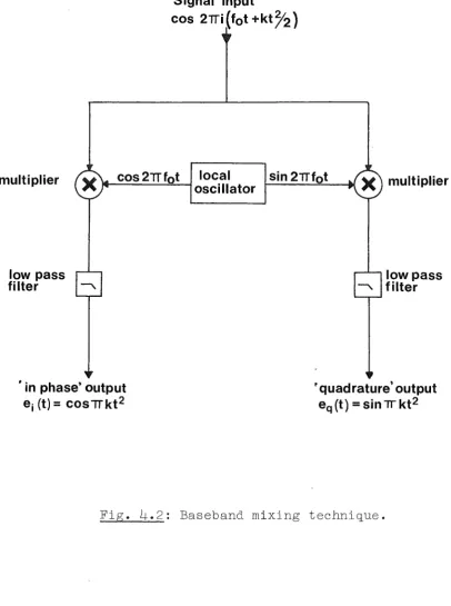
original signal (i.e. both the amplitude and phase) are preserv-ed, this problem of spectral foldover may be avoided. Fig. 4.2 illustrates a method by which this can be accomplished.
This arrangement operates as follows. A local oscillator is provided with two outputs, both at a frequency of f
0, but differing in phase by 90°. The chirp signal is ~ixed with each of these outputs, and the products are lowpass filtered to
retain only the difference terms. The outputs of these filters will be of the same form, but differing in phase by 90°, and may be envisaged as the real and imaginary parts of the
original signal, shifted down to zero frequency. The ability to distinguish positive and negative frequencies will not be lost, since an input to the mixer of exp 2ni(f
0+f1) will appear at the outputs as
=
cos {2nfJand
whereas an input of exp 2ni(f
f0-6fj2 f0 f0+.6.fj2
FREQUENCY
.
-6.V2 0 Af/2
FREQUENCY
t of baseband mixing on signal spectrum •
H::>
Signal Input
cos 2Tri (tot
+kt~2)
multiplier cos2Tif0t local sin 21Tf0t
oscillator
low pass filter
• in phase· output ei (t)
=
COS1Tkt2low pass filter
'quadrature' output eq (t) =sin lT kt2
[image:50.595.87.494.201.747.2]and e ( t)
q
=
the negative sign in the quadrature, or imaginary channel indicating a negative frequency.
The two outputs from the mixer may thus' be regarded as the real and imaginary parts of a complex signal, i.e.
e (t)
=
e. (t) + ie (t)l q ( 4. 14)
If these outputs are sampled simultaneously, the pairs of
samples so obtained would form a set of complex numbers, which would be suitable for processing by the computer.
The operation of the computational filter may now be described in more detail. The input signal to the filter will be of the form
e ( j)
=
( 4. 15)where k is the rate of frequency modulation of the chirp signal
j
=
(0,1,2 .•. N-1)t is the sampling interval. s
Note that this signal is at 'baseband', and that the samples, e(j), are complex.
The discrete spectrum of this signal will be denoted by E(n), where 0 ~ n < N-1. The filter function, given in
contin-uous form in equation (4.11) will be described in discrete form by
Y (n)
c
=
W(n)
where Y (n) and W(n) are the discrete formulation equi-c valents of the functions Y (f) and W(f). The spectrum of the
c
filter output, given in continuous form in equation (4.10) will become
E , (n)
=
Y (n) .E(n)OW C
= W (n) 0 < n < N-1 (4.17)
and of course the corresponding time-domain relationship is
e OW I ( j )
=
W ( j ) 0 < j < N-1 ( 4. 18) Operation of the processing filter first requires that the outputs from the baseband mixer be sampled by the A-D converter, and an FFT performed on these samples. The complex spectral weights E(n) produced by the transform are then each multiplied by the corresponding complex Y (n) to yield E , (n) (i.e.c ow
E , (1)
=
E(l) .Y (1) etc.). These products are thentransfer-ow c
med by an inverse FFT to give the processed time series e , (j). Fig. 4.3 should help clarify this description.
OW
Another important effect of baseband mixing should be recognised. Whereas without mixing, the weighting function needed to be centred about f
0 in order to encompass the signal spectrum, i t now requires to be centred about zero frequency. This implies that rather than being a pulse at frequency f0 with an envelope of w(t), the output is now simply a single
in phase input cos kt2f2
A-D
...
conver- ... ter
I
~E(o)
E(l)quadrature input
1~1--::::
A-D
fs ----~
conver-ter
FFT
E(n) E(N -I)
· YcCo) ·Yc (I) - - ~ - - - ·Yc(n) -- - - ·Yc(N~D
u
. .
. .
.
W(o)
....
r,
w(o)
rwmi\1/
,
,
W(t) W(n) W(N -t)
~ .J
IFFT
W(l) w{n) w(N -I)
..
,,
,
~
COMPLEX AMPLITUDES OF COMPRESSED PULSE [image:53.595.47.553.136.833.2]FREQUENCY DOMAIN TIME DOMAIN
W(f)
w(t)
~0
f t
wtf}
w'(t)
~
0
0 f
t
4.4 APPLICATION TO REAL TARGETS
The preceding analysis has always used, as an input to the processing filter, a signal e(t) consisting of a single chirp of unit amplitude and zero phase, centred about time t
=
0. Now, of course, a real radar return consists of a number of overlapping chirps, each having its own amplitude, phase, and time of arrival. A limiting case of this occurs in theionosphere, where the target is often of a distributed nature. For any signal processing method to be viable, i t must preserve these three parameters of each chirp throughout the processing filter.
Before an analysis of how the proposed filter will handle real radar returns can be made, certain aspects of discrete Fourier transforms must be understood. If H(n) denotes the Fourier transform of an arbitrary time series h(j), then the
following properties hold:
1. A delay, or shift, in the time domain is equivalent to a linear added phase in the frequency domain. That is,
h(j-k)
~
H(n)exp{-2~ikn/N)
(4.19)where in this case the time signal has been delayed by k sampling intervals
and N is the total number of samples.
2. A constant phase change in the time samples produces an equivalent constant phase change in the frequency domain, i.e.
h(j). exp ie
DFY
H.(n). exp iewhere
e
is a constant.This follows directly from the linearity property of Fourier transforms.
An expression may now be derived for the output of the processing filter when excited by a simulated radar return from a point target, that is, a chirp of arbitrary amplitude and phase, delayed by an arbitrary amount of time, say m sampling intervals.
Such a signal would be described by
2
f ( t)
=
jt-mt
l
k (t-mts)A rect
l
T s_j exp{2ni[f0(t-mts) + 2 + ¢]} ( 4. 21) where A is the amplitude of the signal¢ is the phase of the signal, taken with respect to an arbitrary zero
ts is the sampling interval of the A-D converter.
Alternatively,
f (t)
=
Ae ( t-mt ) . exp (2ni¢) swhere e(t) is defined in equation (2.1).
(4.22)
If f(t) is mixed to baseband and sampled, the discrete function so obtained is given by
f(j)
=
A.e (j-m) .exp(2ni¢) (4.23)where e(j) is defined in equation (4.15). The Fourier transform of this would be
F(n)
=
A.exp(2ni¢).E(n) .exp(2nimn/N) (4.24)using properties 1 and 2 given earlier.
Y c (n) F (n)
=
A. exp ( 2 ni ¢) . exp ( 2 nimn/N).Y c (n).E (n)=
A. exp ( 2 ni ¢) . exp ( 2 nimn/N).W (n) (4.25)since Y (n)~(n)
=
W(n) from equation (4.16). cA final inverse Fourier transform 0n this will yield as an output from the filter,
f
0w1 (j)
=
Aw(j-m). exp(2ni¢) (4.26)which is a replica of e 1 (j), the output pulse obtained from ow
an input of e(t), except that i t has been time-shifted by m sampling periods, has an amplitude A, and a phase of ¢.
Thus the composite filter, Y (n), fulfils the conditions c
required by a radar signal processing filter outlined at the beginning of this section. It is easy to generalise the preceding treatment to a case where the input to the filter consists of radar returns from Q targets, each producing an echo of amplitude A , a phase ¢ , and delayed by m sampling
q q q
intervals. The input signal would be a linear combination of all these individual echoes, or
e ( t)
c
Q
= L A e(t-m t ) exp(2ni¢ )
q=l q q s q (4.27)
and by a reasoning similar to the preceding case, the output of the processor would be
Q
ecow 1 (j) = L A w(j-m t ) exp(27ri¢ )
q=l q q s q (4. 28)
4.5 COMPUTER SIMULATION OF THE FILTER
The preceding mathematical analysis indicates the validity of the proposed signal processing method; however, as an
additional confirmation of its performance a simulation of its use was implemented on the University's B6700 computer.
Firstly, the digitized expression for the chirp signal, given in equation (4.15) was evaluated over a range of j, and the numbers so obtained were transformed by an FFT routine to give the complex spectral coefficients, E(n). A weighting function was then selected (the Hamming function in this case) and the coefficients the filter function determined
according to the equation
Y (n)
c
W (n)
E (n) ( 4. 16)
the division, i t will be remembered, is complex. Various input signals were then treated by this lter according to
method depicted in Fig. 4.3.
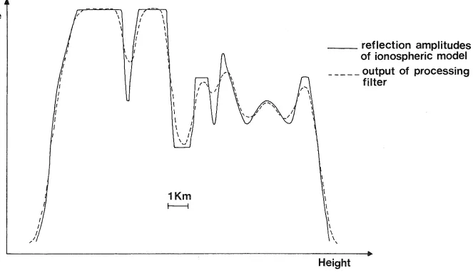
A large number of different signals were processed; in order to test every aspect of the processing filter, and to try and find any problems which might occur in the processing of ionospheric returns. Some examples these signals were:
signals with a number of overlapping and non overlapping chirp pulses (to test the resolution of the system}
signals of varying phase and amplitude
signals with delays that were non-integral multiples of the sampling frequency